DNA Subway
![]()
Goal
DNA Subway is an educational bioinformatics platform developed by CyVerse.
It bundles research-grade bioinformatics tools, high-performance computing, and databases into workflows with an easy-to-use interface.
"Riding" DNA Subway lines, students can predict and annotate genes in up to 150kb of DNA (Red Line), identify homologs in sequenced genomes (Yellow Line), identify species using DNA barcodes and phylogenetic trees (Blue Line), examine RNA-Seq datasets for differential transcript abundance (Green Line), and analyze metabarcoding and eDNA samples using QIIME (Purple Line).
Prerequisites
In order to complete this tutorial you will need access to the following services/software
| Prerequisite | Preparation/Notes | Link/Download |
|---|---|---|
| CyVerse account | You will need a CyVerse account to complete this exercise | Register |
| DNA Subway Access | DNA Subway access is by request access | Check or request access: CyVerse User Portal |
DNA Subway Basics and Logging in to Subway
DNA Subway is designed to be a classroom-friendly approach to bioinformatics. Unlike most CyVerse platforms, you can even use Subway without registering for a CyVerse account. We do encourage you to register however, only work from registered users can be saved. DNA Subway uses the same open-source bioinformatics tools used by researchers. See a complete list of the tools provided in the Subway pipelines.
Some things to remember about the platform
Registered user and Guest user account types
- DNA Subway access must be requested through the CyVerse user portal. You can check if you already have access, or request access by logging into the portal and visiting the My Services page. If DNA Subway is not listed, click on Available services to request access.
- Guest users will not have their worked saved beyond a single DNA Subway session. They are also disallowed from using one of the gene predictors (FGenesH) in the genomic annotation pipeline (Red Line).
- We suggest that every student using DNA Subway obtain their own account.
Sample Datasets and reference data
All Subway lines accept user data and also have sample data that can be immediately used to create a project.
- Red Line - Genome Annotation: Samples of plant and animal genomes that can be used in annotation projects
- Yellow Line - TARGeT Search for transposons and other DNA Sequences: Several model plant genomes
- Blue Line - DNA Barcoding and Phylogenetics: Sample sequence from plant, animal, fungal, and bacterial barcoding regions; human mitochondrial DNA sequence
- Green Line - RNA-Seq for differential expression: Sample high-throughput reads from RNA-Seq experiments
If there is a reference data set or sample sequence you would like added, you can contact CyVerse using the DNA Subway Contact page
Public and private projects - DNA Subway projects are private by default, but can be shared by making them public. Public projects are searchable and are a great way to share data or present analysis for grading in a classroom project.
Logging into DNA Subway as a registered user
- Access the DNA Subway website at https://dnasubway.cyverse.org/
-
If you wish to use DNA Subway as a guest click 'Enter As Guest'
Note
When using DNA Subway as a guest, you will be able to work only on the Red, Yellow, and Blue lines. Additionally, some Red Line functionalities will be disabled. Finally, after logging out, or a period of inactivity (\>\~ 30 min) you work will be discarded. -
Enter your CyVerse username and CyVerse password.
Logging into DNA Subway as a guest user
- Access the DNA Subway website at https://dnasubway.cyverse.org/; click 'Enter as Guest'
Accessing Saved Private and Public DNA Subway Projects
DNA Subway projects are automatically saved for registered users. By default, Subway projects are private upon creation and visible only to you. You may make project public, in which case users will have the ability to view those projects, but may not edit those projects.
Accessing Private Projects
-
Access the DNA Subway website at https://dnasubway.cyverse.org/
-
Upon login, you will see a listing of your private projects. Access the project by clicking the project title.
-
From any DNA Subway page, you may access private projects by clicking the 'My Projects' button on the navigation menu on the left side of the page.
Distinguishing Lines
All projects in DNA Subway are associated with the color of their respective DNA Subway lines, and with a project ID number.
You may see the comments and species associated with the project
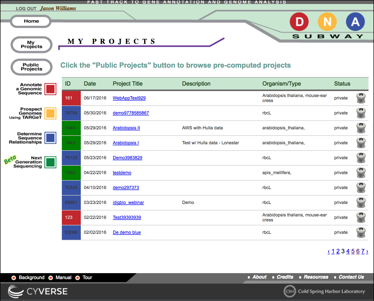
Deleting a project
To delete a project, click the 'trash can' icon. Once deleted, all data related to that project will be lost and unrecoverable.
Accessing Public Projects
-
Access the DNA Subway website at https://dnasubway.cyverse.org/; login to Subway or enter as a guest user.
-
On the navigation menu on the left side of the screen, click 'Public Projects'
Sorting and Search
You can sort by project date or type, and you can search for a project by title, organism, or the name of the project owner. When searching, click the double arrow `` to search by your selected term.
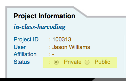
Make a DNA Subway Project Private or Public
- Access the DNA Subway website at https://dnasubway.cyverse.org/; login to Subway.
- Access your selected project by clicking the project title.
- Under the 'Project Information' tab, toggle the project setting to 'Public' or 'Private' as desired.
Walkthrough of DNA Subway Red Line - Genome Annotation
Annotation adds features and information to a DNA sequence -- such as genes and their locations, structures, and functions. A good introduction to annotation can be found in the paper A beginner's guide to eukaryotic genome annotation. We'll also suggest the DNA Subway's primer on annotation evidence. This guide contains an explanation of basic functions for this line, as wellas exercises that might be used in the classroom. Some things to remember about the platform @@ -205,156 +164,115 @@ as exercises that might be used in the classroom.
DNA Subway Red Line - Create an Annotation Project with Apollo
transition away from Java
DNA Subway is transitioning away from the original Java-based Apollo software as most popular web browsers will no longer support Java. The new Apollo is Java-free.
- Log-in to DNA Subway - unregistered users may 'Enter as Guest'
- Click 'Annotate a genomic sequence.' (Red Square); select the 'Web Apollo' version
-
For 'Select Organism type' choose 'Animal' or 'Plant' and then select the appropriate subtype. The 'Select Organism' step will load appropriate sample sequences and will also adjust the models used in the de novo gene finding process.
-
For 'Select Sequence Source' select a sample sequence.
Apollo support
Currently, the Java-free Apollo version of Subway does not support upload of a custom DNA Sequence.
This feature is coming soon, but we will help you upload custom genomes/regions for your use in the classroom
- (Optional) If you have a GFF file of annotated features, you may load these import these annotations from the Green Line, or from a custom GFF file.
- Name your project and organism (required) and give a description if desired. Click 'Continue' to proceed.
Example Exercise - Project Creation: Arabidopsis ChrI
In this and subsequent steps, we will annotate a 75KB section of Arabidopsis chromosome I. 1. Log-in to DNA Subway - unregistered users may 'Enter as Guest'. 2. Click 'Annotate a genomic sequence.' (Red Square); select the 'Web Apollo' version. 3. For 'Select Organism type' choose 'Plant' and then 'Dicotyledon'. 4. from 'Select a sample sequence' chose 'Arabidopsis thaliana (mouse-ear cress) chr1, 75.00 kb'. 5. Provide your project with a title, then Click 'Continue.'
Sequence
You can view your DNA sequence by clicking the 'Sequence' link in the 'Project Information' tab at the bottom of the page.
DNA Subway Red Line - Find and Mask Repetitive DNA
One you have created a Red Line Project, you may begin the process of generating and assembling predictions and evidence that can be used to annotate genes. 1. Click 'RepeatMasker' 2. When 'RepeatMasker' turns 'green' and the icon displays a 'V' (view); click 'RepeatMasker' again to view results.
{width="300px" height="200px"}
Example Exercise - Repeat Masking: Arabodopsis ChrI
- Example Sequence: Arabidopsis thaliana (mouse-ear cress) ChrI, 75 kb
- Tool(s): RepeatMasker
- Concept(s): Non-coding DNA, sequence repeats, mobile genetic elements (transposons)
Following the RepeatMasking steps for the Arabidopsis ChrI sample above, answer the following discussion questions: 1. How many hits were detected in your sample? 2. RepeatMasker reports the length of the repetitive sequences (Length) as well as the class (Attributes). - What is the average length of sequences identified as "simple repeats"? - What is the average length of sequences identified as "low complexity"? 3. What is the total percentage of repetitive DNA in your sequence? (Sum of the length of all repetitive sequence / sequence length (75 kb)
Some Useful Definitions for Repetitive Sequences
-
Simple repeats: 1-5bp repeats (e.g. repetitive dinucleotides 'AT' etc.)
-
Low Complexity DNA: Poly-purine/ poly-pyrimidine stretches, or regions of extremely high AT or GC content.
-
Processed Pseudogenes, SINES, Retrotranscripts: Non-functional RNAs present within genomic sequence.
-
Transposons (DNA, Retroviral, LINES): Genetic elements which have the ability to be amplified and redistributed within a genome.
Additional Investigation: In the results table under 'Attributes' each repeat sequence is labeled "RepeatMasker#-XXX" The '#' is the ordinal number of the hit, the XXX is the class of DNA element (e.g. "Simple_repeat" or "Low_complexity"). There are other types of repetitive elements such as transposons and pseudogenes (e.g. Helitron and COPIA) Use online resources to learn more: (http://gydb.org/index.php/Main_Page).
DNA Subway Red Line - Making Gene Predictions
De novo gene predictors can be run on a sample sequence to generate predictions of gene structure and location based solely on the sequence nucleotides.
- Click on one or more gene prediction tools under the 'Gene Prediction' stop. to view the results table, click the gene predictor again once the indicator displays 'V' (view).
Example Exercise - Predict Genes: Arabidopsis ChrI
- Example Sequence: Arabidopsis thaliana (mouse-ear cress) ChrI, 75 kb
- Tool(s): Augustus, FGenesH, Snap, tRNA Scan
- Concept(s): Genomic DNA, Gene Structure, Canonical sequences
Following the gene prediction steps for the Arabidopsis ChrI sample above, answer the following discussion questions:
-
Look at the 'Type' column in the gene prediction report. Considering the Augustus results, find the 6th gene prediction (hint: AUGUSTUS006;ID=g6) and then locate the first mention of the term 'gene' and copy down the gene's 'start' (i.e. the starting basepair). Note the number of times you see the term 'exon' (i.e. number of exons predicted).
Gene Predictor Exon Start (bp) Exon Stop (bp) Augustus 23456 23684 Augustus Augustus Augustus Augustus -
Based on the chart, did all the gene predictors yield genes starting at the same location? Did all the gene predictions have the same number of exons?
- Looking at the number of results returned by tRNA Scan, why are they so different from results made by other predictors? Are their places in the genome where tRNAs are more or less densely concentrated?
Additional Investigation: Look for the background link at the bottom of the DNA Subway home page and review the section entitled 'Gene Finding'.
DNA Subway Red Line - Visualize predicted genes in a Genome Browser
A genome browser is an essential tool for visualization genomic data in context. The integrated JBrowse genome browser will allow you to see the visualized gene predictions generated so far.
- Click 'JBrowse' and allow browser to load.
-
Zoom into a region (for example, paste the region 1:3740638..3749063 into the location window.
Tip
- JBrowse will load multiple tracks of data. Since the entire genome is loaded, we recommend using the 'highlight a region' feature to help keep your place. You may also wish to record the coordinates you are viewing as shown in the coordinates window. - You may also adjust the settings for a particular track by clicking on the track name. - Right-click on any gene to view additional details about that gene. {width="400px" height="250px"} -
Examine gene details by double-clicking on a gene to select; then right-click to open the 'View Details' menu.
- To view more tracks, click on 'Full-Screen View' in the upper-left of the JBrowse window to see any additional tracks available.
Useful Definitions
Genome Browser: A GUI (Graphical User Interface) for viewing biological information. GBrowse (DNA Subway's Browser) is "designed to view genomes. It displays a graphical representation of a section of a genome, and shows the positions of genes and other functional elements. It can be configured to show both qualitative data such as the splicing structure of a gene, and quantitative data such as microarray expression levels." [citation]
Track: The individual regions of the display where information imported into the browser. For each type (or source) of information, there is usually an associated track.
Example Exercise - Visualize predicted genes: Arabidopsis ChrI
- Example Sequence: Arabidopsis thaliana (mouse-ear cress) ChrI, 75 kb
- Tool(s): Local Browser (JBrowse)
- Concept(s): Gene orientation/structure, transposons, chromosome organization
Following the gene browser steps for the Arabidopsis ChrI sample above, answer the following discussion questions (the locations of the genes are given in parentheses and can be pasted into the browser):
Considering the following genes:
- BFN1-201 (1:3748591..3753070)
- SCAMP5-201 (1:3744556..3749035)
- STP1-201 (1:3776366..3780845)
-
At1G11270.2 (1:3780041..3789000)
-
Do all the gene predictors agree with each other?
- Which gene predictions seem to match the Ensemble genes most closely?
DNA Subway Red Line - Search Databases using BLAST
DNA Subway searches customized versions of UniGene and UniProt that contain only validated plant proteins, and are free of predicted or hypothetical proteins.
- Click 'BLASTN'; wait until the flashing icon displays 'V' (view)
- Click 'BLASTN' again to view the results.
- Click 'BLASTX'; wait until the flashing icon displays 'V' (view).
- Click 'BLASTX' again to view the results.
- Click on 'JBrowse' and then click 'Full-screen View' in the upper-left.
- In the 'Available Tracks' menu, add the Blastn and Blastx tracks.
Useful Definitions
**Some Useful Definitions**
- BLAST: Basic Local Alignment Search Tool (BLAST) is an algorithm that search databases of biological sequence information (e.g. DNA, RNA, or Protein sequence) and return matches. The BLASTN program is specific to nucleotide data, and the BLASTX algorithm works with sequence data translated into amino acid sequences.
- UniGene: A database of transcript data, "each UniGene entry is a set of transcript sequences that appear to come from the same transcription locus (gene or expressed pseudogene), together with information on protein similarities, gene expression, cDNA clone reagents, and genomic location." [citation]
- cDNA: DNA produced by reverse transcribing mRNA using reverse transcriptase. cDNAs are used to investigate mRNA within a biological sample.
- ESTs: "Small pieces of DNA sequence (usually 200 to 500 nucleotides long) that are generated by sequencing either one or both ends of an expressed gene. The idea is to sequence bits of DNA that represent genes expressed in certain cells, tissues, or organs from different organisms." [citation]
Example Exercise - Search Databases using BLAST: Arabidopsis ChrI
- Example Sequence: Arabidopsis thaliana (mouse-ear cress) ChrI, 75 kb
- Tool(s): BLASTN, BLASTX, Upload Data
- Concept(s): RNA, cDNAs, ESTs, Biological Databases
Following the BLAST steps for the Arabidopsis ChrI sample above, answer the following discussion questions (the locations of the genes are given in parentheses and can be pasted into the browser):
- Both BLASTN and BLASTX returns the 'Length' of your resulting matches. Do you notice differences in the average lengths of BLASTN and BLASTX matches? Explain.
- Under 'Type' both BLASTN and BLASTX returns 'match' and 'match_part.' 'Match' is describing the overall length of a single match, but individual significant matches may be fragmented, i.e. 'match_part.' Do BLASTN and BLASTX return 'match' and 'match_part' results in different frequencies? Explain.
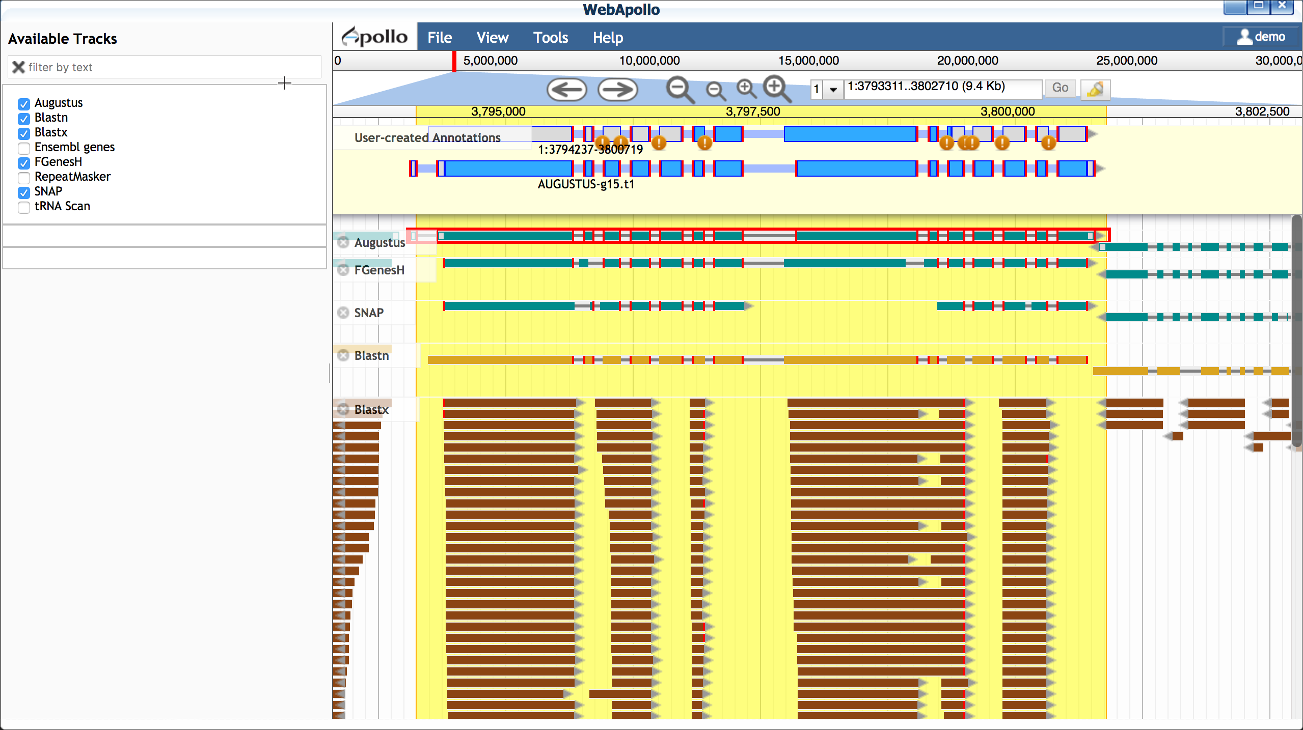
DNA Subway Red Line - Build Gene Models using Apollo
Apollo is an extension of JBrowse which allows the user to build and edit gene models. Apollo has a number of features but in this tutorial, we will give brief intro covering the conceptual steps.
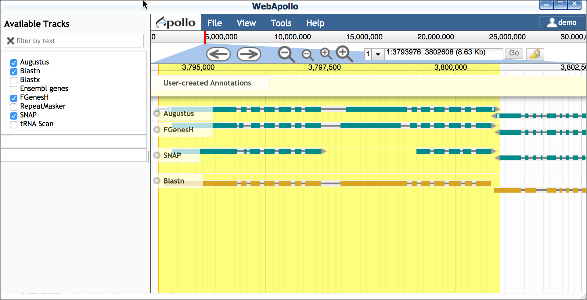
A. Import Blastn model to match for transcript length Blast searches are matched against UniGene(blastn) and UniProt(blasts). UniGen models are derived from cDNA and ESTs (transcriptome evidence) produced by experiment.
- Open Apollo and zoom into a region of interest (e.g. 1:3793981..3802033)
- Ensure at least the following tracks are selected (on):
- Augustus (and other gene predictors: FGenesH, SNAP, etc.)
- Blastn
- Double-click on the Blastn result, and drag this transcript into
the yellow 'User-created Annotations' section.
 {width="400px"
height="250px"}
{width="400px"
height="250px"}
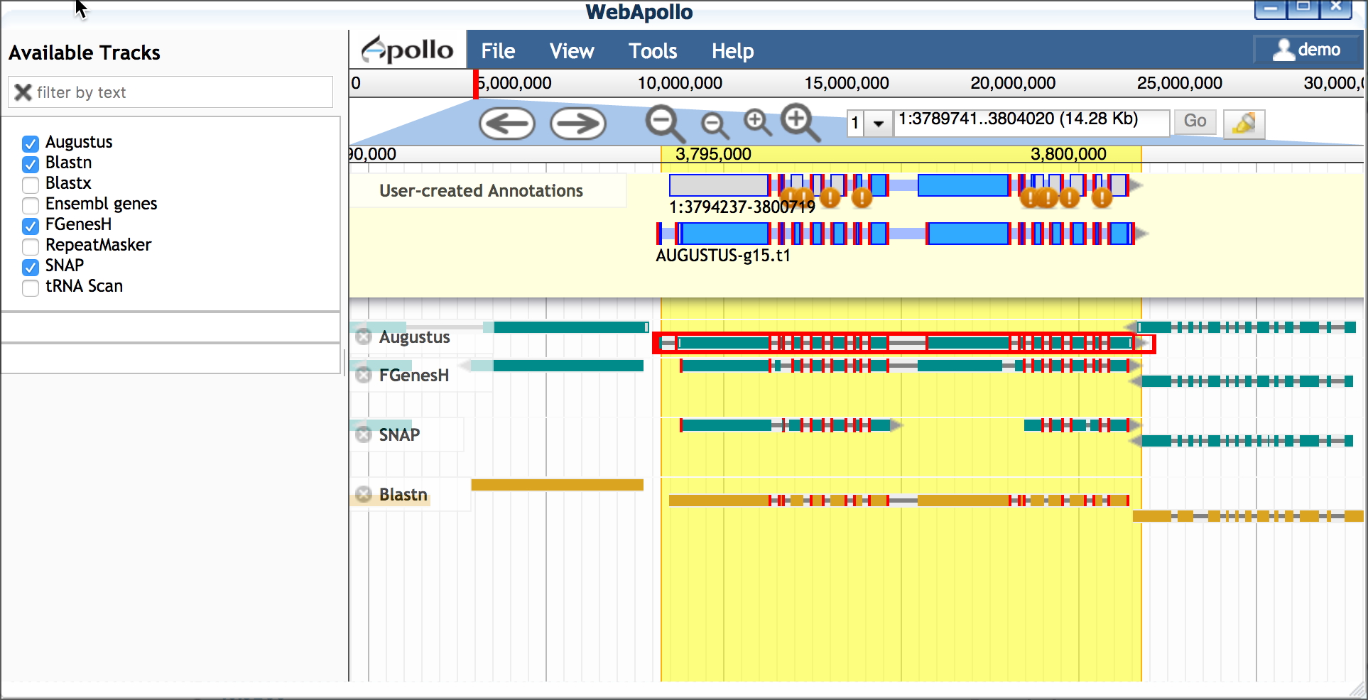
B. Select a scaffold model Use transcriptome evidence (UniGene - BLASTN) to select the best possible gene model for a scaffold. If no gene model exists or significantly reflects the UniGene model, use the UniGene model itself as a scaffold.
- Drag a plausible model into the yellow 'User-created Annotations' - in this case we will choose the Augustus model; double-click the Augustus model to select the entire model and drag into 'User-created Annotations'.
- Adjust the Augustus model to match the 5' and 3' configuration
of the blastn model
- Delete the extraneous 5' exon (single-click to select; right-click to delete)
- Adjust the new 5' end to match the length of the blastn-derived transcript
- Adjust the 3' end of the Augustus-derived model (single-click
to select; use your cursor/mouse to adjust the model length)
C. Edit model for splice sites and variants Protein and EST data can be used to examine possible alternative transcripts. Proteins give clues to the actual length of the translated protein at that locus and its reading frame. Like full length cDNAs, ESTs give valuable information on transcript diversity. ESTs are generated by high throughput methods, and although the data may be fragmentary, it may capture biologically relevant information about splice variants.
-
Turn on the blastx track
-
Examine the additional evidence to consider making adjustments to your Augustus-derived model. If you wish to make additional isoforms of your gene:
- Double-click to select the entire Augustus-derived model
- Right-click on the model to duplicate
- Make adjustments to the model as desired
You also have the option of adding additional EST evidence. For the Arabodopsis 75KB section, we have prepared a selection of EST data. You will need to close Apollo to load this data.
- Download the Arabidopsis ESTs for this region to your computer from this link
- Click on 'Upload Data'; under "Add DNA data in FASTA format" upload the EST file from the link in step 1.
- Click on 'User BLASTN' to align the ESTs to this section of the Arabidopsis genome
- Open 'Web Apollo'. The "Blastn User" track should be loaded.
You may move this track to a convenient position on the browser
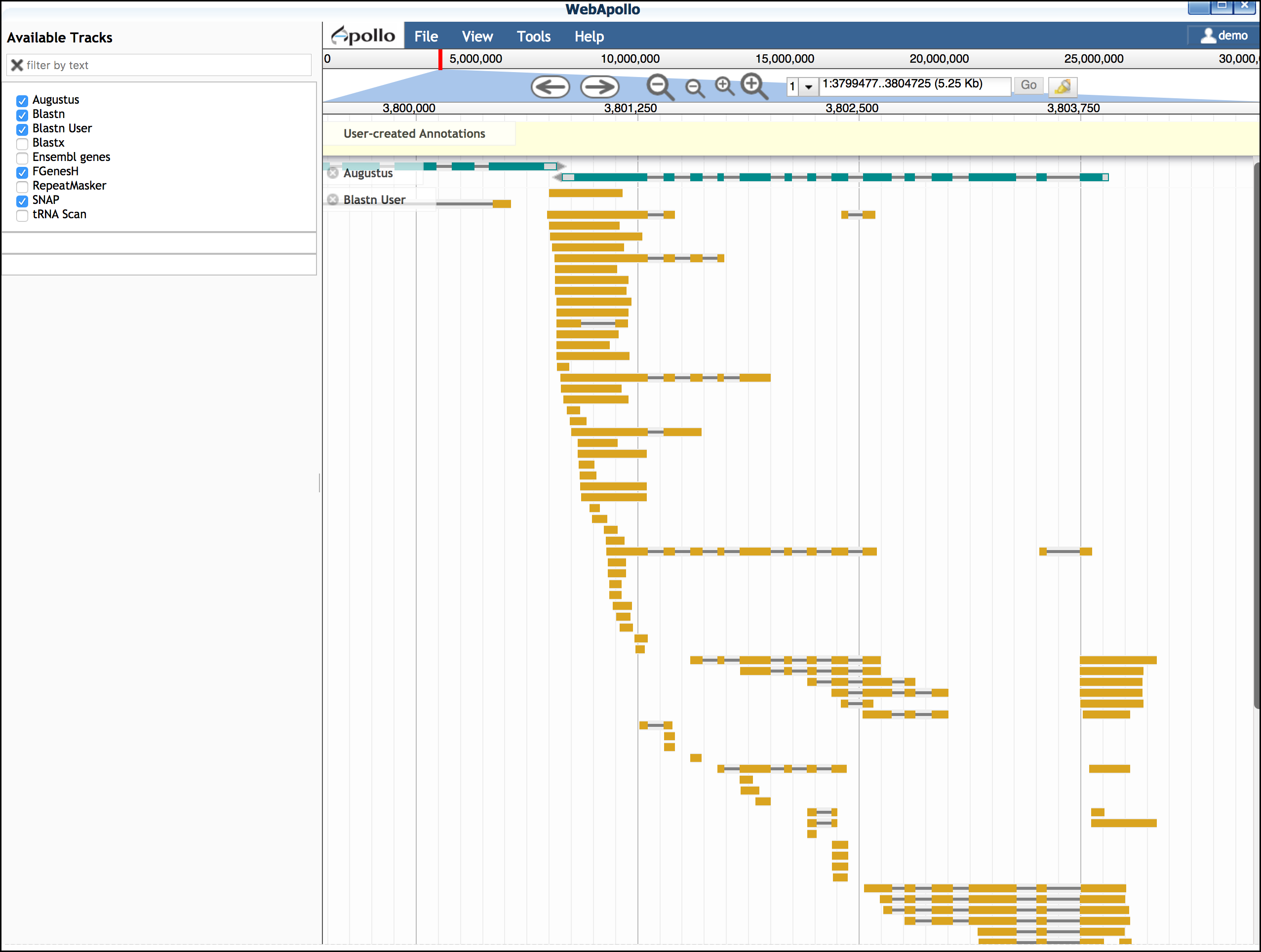
While EST evidence is always incomplete, these sequences can help you determine features of the gene model.
Learn More about Gene Evidence
- J.Craig Venter on ESTs
- "Dynamic Gene" Evidence animation (requires Flash)
D. Determine translation start/stop sites After making your adjustments, you can confirm that your gene model(s) represents the longest possible transcripts:
- Double-click the model; right-click and select 'Set longest ORF'
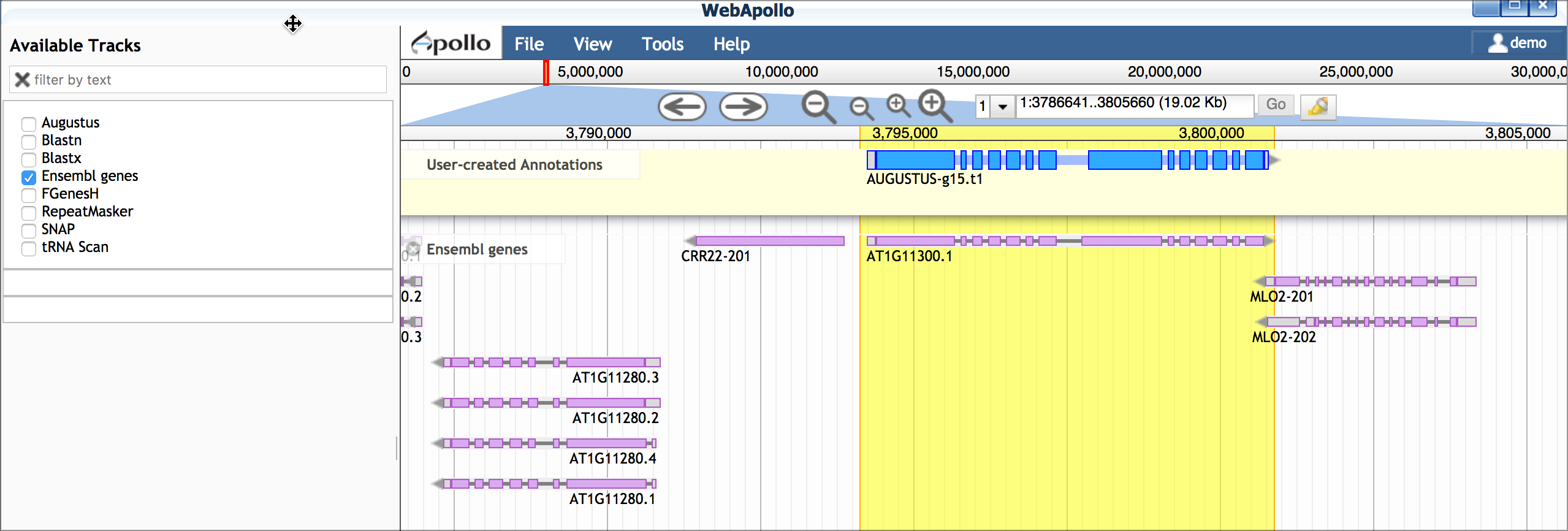
E. Compare gene model(s) with existing annotations After making your gene models you can compare them with existing annotations by turning on the 'Ensemble genes' track. In this case, our work confirms the first gene model made, but a potential isoform supported by blastx data is likely incorrect.
Example Exercise - Build Gene Models using Apollo: Arabodopsis ChrI
- Example Sequence: Arabidopsis thaliana (mouse-ear cress) ChrI, 75 kb
- Tool(s): Apollo
- Concept(s): Synthesizing multiple lines of evidence
Following the Apollo steps for the Arabidopsis ChrI sample above, answer the following discussion questions (the locations of the genes are given in parentheses and can be pasted into the browser):
- Try annotation of the following genes and take notes on your
annotation ( right-click on the gene model, open the 'Information
Editor' and scroll down to the comments section to enter
comments). How do your annotations compare with the Ensembl
annotations?
Genes to try:
- AT1G11270.2 (1:3781511..3790520)
- STP1-201 (1:3776261..3785270)
- T28P6.11-201 (1:3762877..3764678)
Walkthrough of DNA Subway Yellow Line - Sequence Detection
Genome prospecting uses a query sequence (DNA or protein of up to 10,000 base pairs/amino acids) to find related sequences in specific genomes or in a database. A major purpose of genome prospecting is to identify members of gene or transposon families. DNA Subway uses the TARGeT workflow, which integrates BLAST searches, multiple sequence alignments, and tree-drawing utilities. Yellow line uses TARGeT (Tree Analysis of Related Genes and Transposons) uses either a DNA or amino acid 'seed' query to: (i) automatically identify and retrieve gene family homologs from a genomic database, (ii) characterize gene structure and (iii) perform phylogenetic analysis. Due to its high speed, TARGeT is also able to characterize very large gene families, including transposable elements (TEs). [citation]
Some things to remember about the platform
- Yellow Line will return sequences that would normally be excluded from a BLAST search of a genome (e.g. repetitive sequences, transposons).
- Yellow Line is implemented only for plant genomes
DNA Subway Yellow Line - Create a Yellow Line Project
- Log-in to DNA Subway - unregistered users may 'Enter as Guest'
- Click 'Prospect Genomes using TARGeT' (Yellow Square)
-
Select a sample sequence, or paste in a sequence to search for.
Note
DNA Subway Yellow Line is only implemented to search a limited set of plant genomes.
-
Provide your project with a title, then Click 'Continue'
Example Exercise - Project Creation: mPing Mite element to search plant genomes for an active transposon
The mPing MITE element is an example of an active transposon in rice. Transposons are a major class of DNA elements that impact the function of the genome.
- Create a Yellow Line project following the steps above and using the mPing Mite Element (Oryza sativa/Rice)
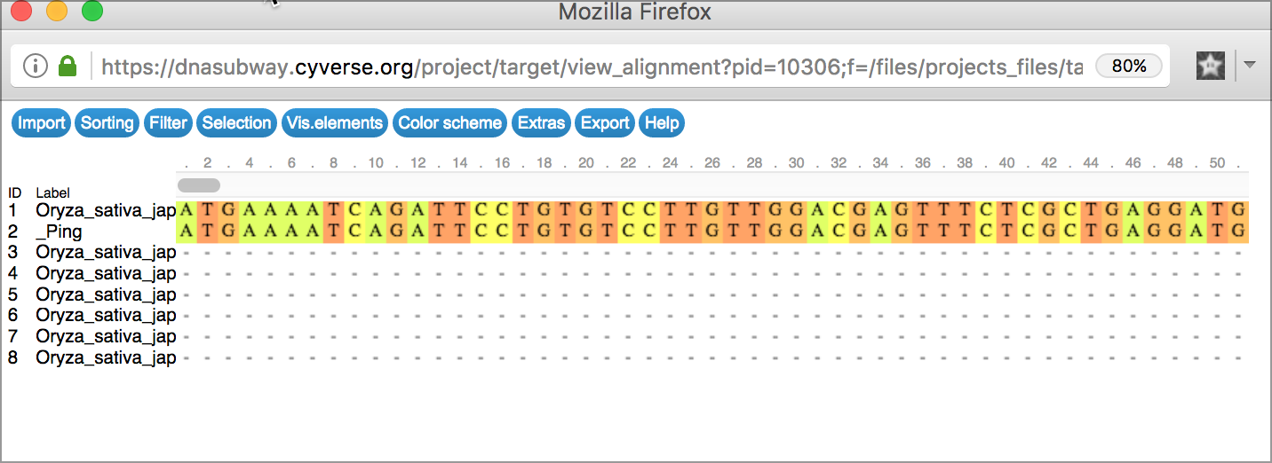
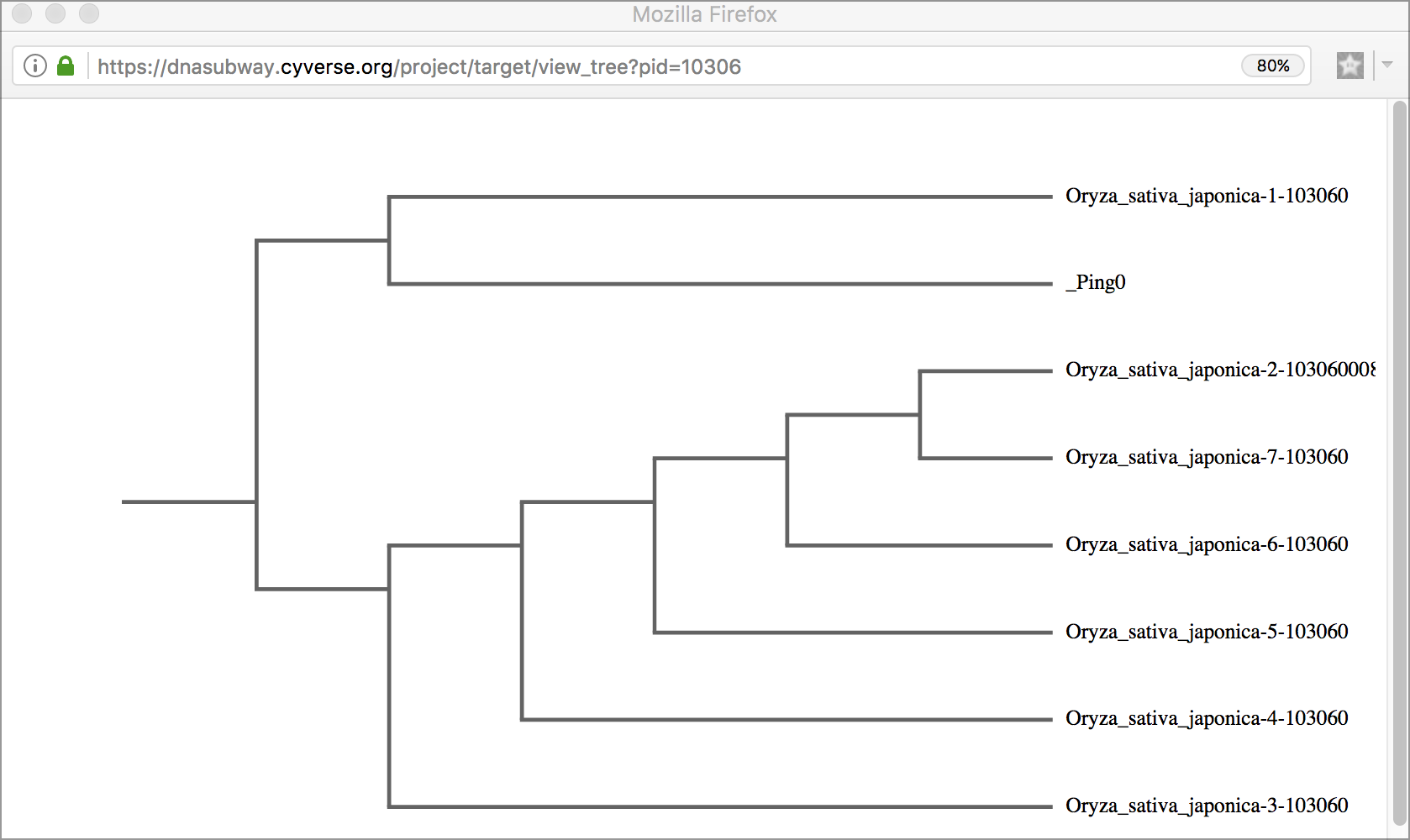
DNA Subway Yellow Line - Search Plant Genomes with TARGeT
- Click and select the genome(s) you wish to search and the click; 'Run' to search those genomes.
- Click the 'Alignment Viewer' button to view the results of the search as a multiple alignment.
- Click the 'Tree Viewer' button to view a tree that will group results by similarity.
Viewer Tips
Alignment Viewer Generates an alignment of all search results
 Tree Viewer Displays the results of sequence matches as a tree, grouped by sequence similarity
yellow_tree
Tree Viewer Displays the results of sequence matches as a tree, grouped by sequence similarity
yellow_tree
Useful Definitions
- Transposons (DNA, Retroviral, LINES): Genetic elements which have the ability to be amplified and redistributed within a genome.
- Non-autonomous transposons: Transposons which lack an active transposase gene, thus requiring help from another transposon to move.
- Autonomous transposons: Transposons which have a functional transposase and can move within the genome.
Example Exercise - Search Plant Genomes: mPing Mite element
- After loading the mPing Mite Element as the query, search the Oryza Sativa genome, and examine the results in the Alignment and Tree Viewers.
- Repeat this analysis with a new project using the Ping transposase gene and the Ping Transposase protein.
Walkthrough of DNA Subway Blue Line - DNA Barcoding and Phylogenetics
You can analyze relationships between DNA sequences by comparing them to a set of sequences you have compiled yourself, or by comparing your sequences to other that have been published in database such as GenBank (National Center for Biotechnology Information). Generating a phylogenetic tree from DNA sequences derived from related species can also allow you to draw inferences about how these species may be related. By sequencing variable sections of DNA (barcode regions) you can also use the Blue Line to help you identify an unknown species, or publish a DNA barcode for a species you have identified, but which is not represented in published databases like GenBank.
Some things to remember about the platform
- Wet lab protocols and other resources are available at http://dnabarcoding101.org/
- The DNA Barcoding 101 site also contains information on low-cost sequencing for U.S.-based educators.
Sample Data
**How to use provided sample data**

In this guide, we will use a mosquito dataset that includes DNA
sequences isolated from mosquito larvae collected from Virginia's
Shenandoah Valley (*"Mosquito dataset"*). There is a complete
two-hour classroom bioinformatics lab with detailed instructions for
instructors and students on QUBES hub
[here](https://qubeshub.org/qubesresources/publications/165/2). Where
appropriate, a note (in this orange colored background) in the
instructions will indicate which options to select to make use of this
provided dataset.

**Sample data citation**: Williams, J., Enke, R. A., Hyman, O.,
Lescak, E., Donovan, S. S., Tapprich, W., Ryder, E. F. (2018). Using
DNA Subway to Analyze Sequence Relationships. (Version 2.0). QUBES
Educational Resources.
[doi:10.25334/Q4J111](http://dx.doi.org/10.25334/Q4J111)

**Video Course**

Here is a video series on analyzing data with DNA Subway using the
above mosquito dataset and lesson:

<iframe width="560" height="315" align="center" src="https://www.youtube.com/embed/videoseries?list=PLRosqf3DDcTFqyPDG04Ed9EjrjaC_UTQo" frameborder="0" allow="accelerometer; autoplay; encrypted-media; gyroscope; picture-in-picture" allowfullscreen></iframe>
Tip
See a Course Source paper with protocols and recommendations for
implementing a Barcoding CURE (course-based undergraduate research
experience): [CURE-all: Large Scale Implementation of Authentic DNA Barcoding Research into First-Year Biology Curriculum](https://www.coursesource.org/courses/cure-all-large-scale-implementation-of-authentic-dna-barcoding-research-into-first-year).
DNA Subway Blue Line - Create a Barcoding Project
- Log-in to DNA Subway - unregistered users may 'Enter as Guest'. !!! Note Only registered users submitting novel, high-quality sequences will be able to submit sequence to GenBank
-
Choose a project type:
- Phylogenetics: build phylogenetic trees from any DNA, protein, or mtDNA sequence)
- Barcoding: DNA Barcoding for plants (rbcL), animals (COI), bacteria (16S), and fungi (ITS).Sample Data
*"Mosquito"* dataset: Select **COI**.3. Under 'Select Sequence Source' select a sequence by uploading either a FASTA file or AB1 Sanger sequencing tracefile; pasting in a sequence in FASTA format, or selecting and importing a trace file from DNALC. If you do not have a file, you may select any of the available sample sequences.
Sample Data
*"Mosquito"* dataset:
From **Select a set of sample sequences** select **Intro to Barcoding Bioinformatics: Mosquitoes**.
4. Name your project, and give a description if desired; click 'Continue.'
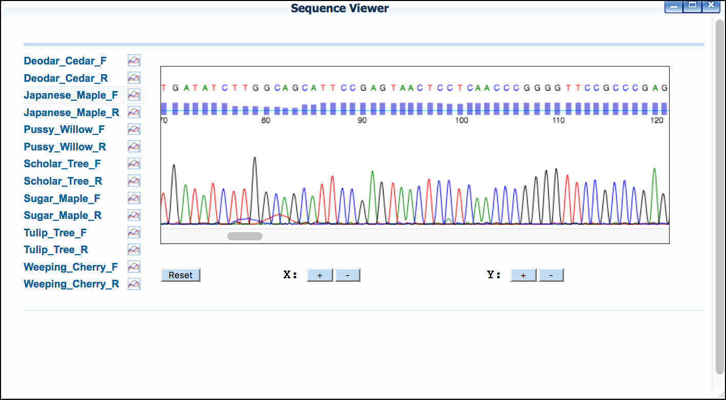
DNA Subway Blue Line - View and Clean Barcoding Sequence Data
A. View Sequencing Trace File
If you provided AB1 trace files, or imported files from DNALC, you will be able to view the sequence electropherogram.
- Click 'Sequence Viewer' to show a list of your sequences.
- Click on a sequence name to show the sequences' trace file.
B. Trim sequence, reverse complement and pair
By default, DNA Subway assumes that all reads are in the forward orientation, and displays an 'F' to the right of the sequence. If any sequence is not in that orientation, click the "F" to reverse compliment the sequence. The sequence will display an "R" to indicate the change.
- Click 'Sequence Trimmer.'
- Click 'Sequence Trimmer' again to examine to changes made in the sequence
- Click 'Pair Builder.'
-
Select the check boxes next to the sequences that represent bidirectional reads of the same sequence set. Alternatively Select the 'Auto Pair' function and verify the pairs generated.
Sample Data
*"Mosquito"* dataset: Click **Try Auto Pairing**. One pair of horsefly sequences and 4 pairs of mosquito sequences will be created. Finally, click `Save`{.interpreted-text role="guilabel"}. -
As necessary, Reverse Compliment sequences that were sequenced in the reverse orientation by clicking the 'F' next to the sequence name. The 'F' will become an 'R' to indicate the sequence has been reverse complimented.
- Click
Saveto save the created pairs.
C. Build a consensus sequence This step remove poor quality areas at the 5' and/or 3' ends of the consensus sequence.
- Click on "Trim Consensus." Once the job is ready to view, click "Trim Consensus" again to view the results. Scroll left and right in the consensus editor window to identify what string of nucleotides from the consensus sequence you want to trim.
- Click on the last consensus sequence nucleotide that you want to trim. A red line will indicate what nucleotides will be removed from the consensus sequences.
-
Click
Trim. A new "Consensus Editor" window will pop up displaying the trimmed sequences.Sample Data
*"Mosquito"* dataset: All of the sequences in this dataset benefit from trimming. Follow the steps above to trim sequences. We recommending trimming at the first and last "grey" (lower quality) nucleotide on the right and left ends.
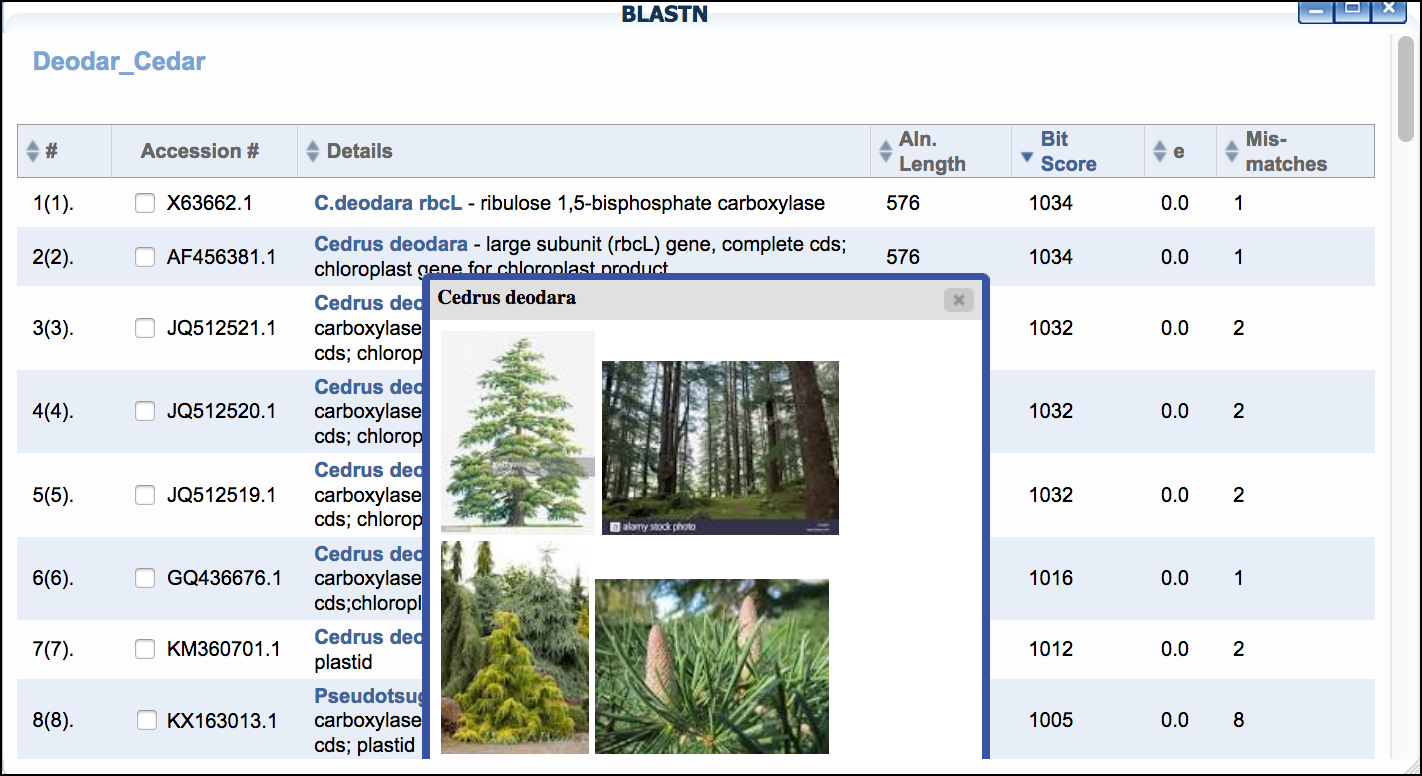
DNA Subway Blue Line - Find Matches with BLAST
DNA Subway Blue Line will search a local copy of a BLAST databases to check for published matches in GenBank.
Tip
At the end of the BLAST results page, you can see the latest update to the DNA Subway BLAST database.
- Click 'BLASTN' then click the 'BLAST' link to BLAST the sequence of interest. When the search is completed a 'View' link will appear.
- Examine the BLAST matches for candidate identification. Clicking the species name given in the BLAST hit will also give additional information/photos of the listed species.
-
If desired, select the check box next to any hit, and click
&Add BLAST hits to projectto add selected sequences to your project.
Sample Data
*"Mosquito"* dataset: We recommend performing a BLASTN search for all samples and saving the top 2 matches to your project for additional analysis (as in Step 3).
DNA Subway Blue Line - Add Reference Data
Depending on the project type you have created, you will have access to additional sequence data that may be of interest. For example, if you are doing a DNA barcoding project using the rbcL gene, samples of rbcL sequence from major plant groups (Angiosperms, Gymnosperms, etc.) will be provided. Choose any data set to add it to your analysis; you will be able to include or exclude individual sequences within the set in the next step.
- Click 'Reference Data.'
- Select sequences of your choice.
-
Click
Add ref datato add the data to your project.Sample Data
*"Mosquito"* dataset: Select **Common insects** and then click `&Add ref data`{.interpreted-text role="guilabel"}.
DNA Subway Blue Line - Build a Multiple Sequence Alignment and Phylogenetic Tree
A. Build a multiple sequence alignment and phylogenetic tree
- Click 'Select Data.'
-
Select any and all sequences you wish to add to your tree.
Sample Data
*"Mosquito"* dataset: We suggest first adding your \"user data\" and building an alignment and tree. You can return to this step later to build additional trees. Once Selected, click `Save Selections`{.interpreted-text role="guilabel"}. Follow the rest of the steps in this section and section B to create your tree. -
Click
Save Selectionsto select data - Click 'MUSCLE.' to run the MUSCLE program.
- Click 'MUSCLE' again to open the sequence alignment window.
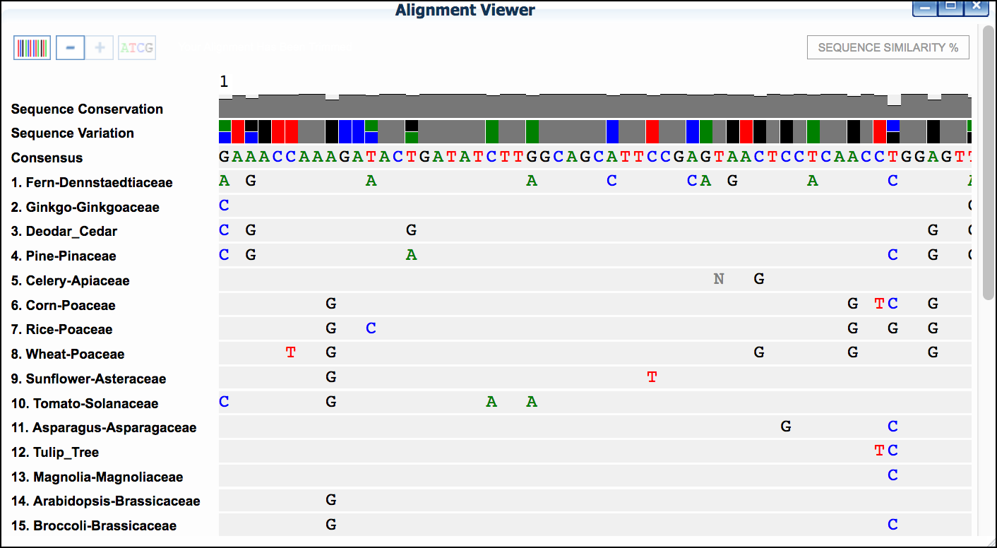
- Examine the alignment and then select the
Trim Alignmentbutton in the upper-left of the Alignment viewer'.
B. Build phylogenetic tree
-
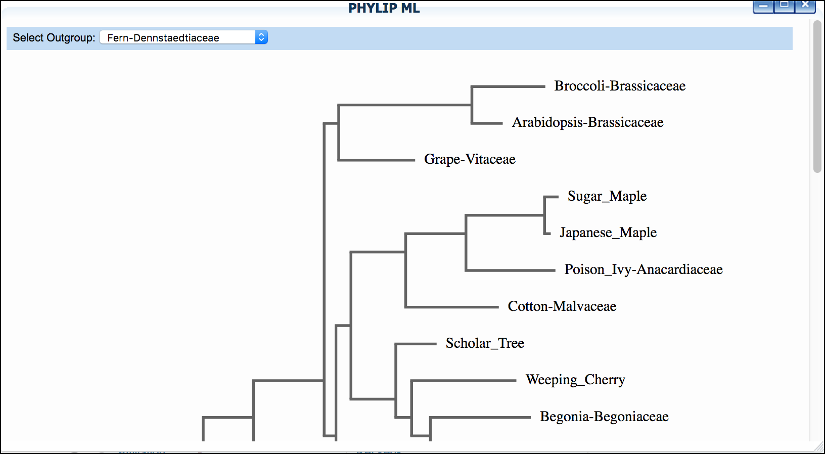
Click 'PHYLIP NJ' and then click again to examine a neighbor-joining tree
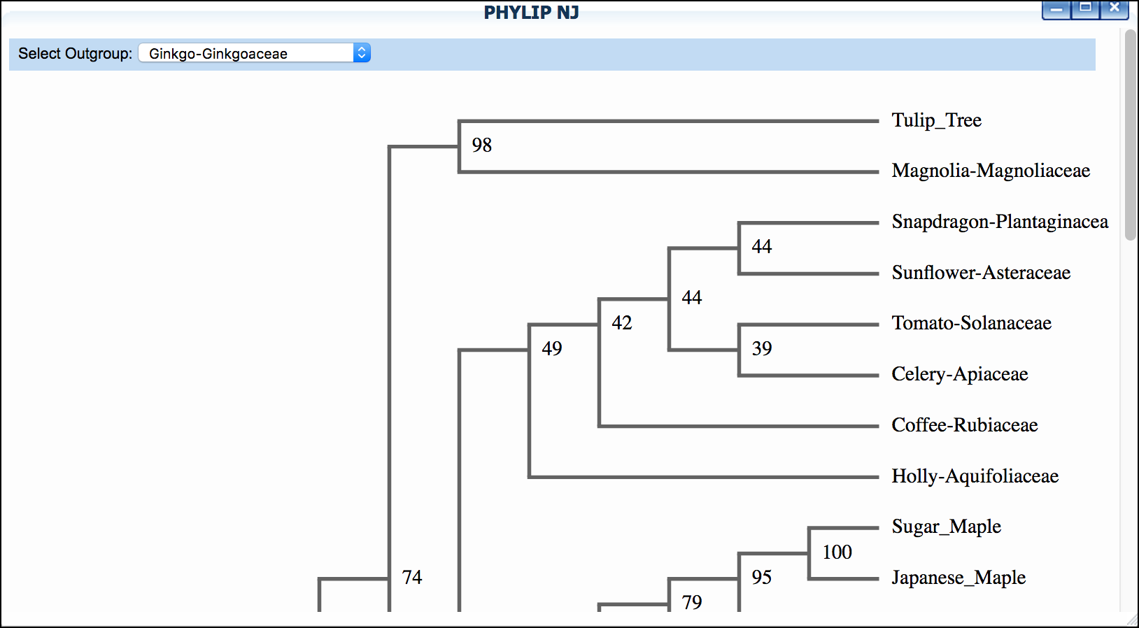
-
Click 'PHYLIP ML' and then click again to examine a maximum-likelihood tree
Sample Data
*"Mosquito"* dataset: We suggest setting "horsefly" as outgroup for both trees.
Walkthrough of DNA Subway Green Line: Kallisto/Sleuth RNA-Seq
The Green Line runs within CyVerse DNA Subway and leverages powerful computing and data storage infrastructure and uses the supercomputer cluster to provide a high performance analytical platform with a simple user interface suitable for both teaching and research. is a quick, highly-efficient software for quantifying transcript abundances in an RNA-Seq experiment. Even on a typical laptop, Kallisto can quantify 30 million reads in less than 3 minutes. Integrated into CyVerse, you can take advantage of CyVerse DNA Subway to process your reads, do the Kallisto quantification, and analyze reads with the Kallisto companion software in an R-Shiny app.
Some things to remember about the platform
- You must be a registered CyVerse user to use Green Line.
- The Green Line was designed to make RNA-Seq data analysis "simple". However, we ask that users thoughtfully decide what "jobs" they want to submit. Each user is limited to a maximum of 4 concurrent jobs running on Green Line.
- A single Green Line project may take a week to process since HPC computing is subject to queues which hundreds of other jobs may be staging for. Additionally these systems undergo regular maintenance and are subject to periodic disruption.
Note
New, faster Green Line
Green Line is now running on Jestream Cloud. This should greatly reduce queue times (The entire running time for this tutorial is about 60 minutes). We have designed Green Line for a lower number of concurrent users (<50), and still recommend teaching using jobs you have made public, and only running the entire workflow when you are working with novel data. Please let us know about your experience: send feedback.
Important: Discontinued Support for Tuxedo Workflow
The Tuxedo workflow previously implemented for the Green Line will has been removed in June 2019. Data and previously analyzed results will still be available on the CyVerse Data Store, however it is not possible to execute new analyses which include Tuxuedo.
Sample Data
**How to use provided sample data**

In this guide, we will use an RNA-Seq dataset (*"Zika infected
hNPCs"*). This experiment compared human neuroprogenetor cells
(hNPCs) infected with the Zika virus to non-infected hNPCs. You can
read more about the experimental conditions and methods in this [reference](https://journals.plos.org/plosone/article?id=10.1371/journal.pone.0175744).
Where appropriate, a note (in this orange colored background) in the
instructions will indicate which options to select to make use of this
provided dataset.

**Sample data citation**: Yi L, Pimentel H, Pachter L (2017) Zika
infection of neural progenitor cells perturbs transcription in
neurodevelopmental pathways. PLOS ONE 12(4): e0175744. [reference](https://journals.plos.org/plosone/article?id=10.1371/journal.pone.0175744).

**Video Course**

Here is a video series on analyzing data with DNA Subway using the above Zika dataset and lesson:

<iframe width="560" height="315" align="center" src="https://www.youtube.com/embed/videoseries?list=PLRosqf3DDcTHLTsiCTT8tnA2ZAfMM5AWb" frameborder="0" allow="accelerometer; autoplay; encrypted-media; gyroscope; picture-in-picture" allowfullscreen></iframe>
DNA Subway Green Line: Kallisto/Sleuth - Create an RNA-Seq Project to Examine Differential Abundance
A. Create a project in Subway
- Log-in to - unregistered users may NOT use Green Line.
- Click on the Green "Next Generation Sequencing" square to start a Green Line project.
-
For 'Select Project Type' select either "Single End Reads" or "Paired End Reads".
Sample Data
*"Zika infected hNPCs"* dataset: Select **Paired End Reads**
4. For 'Select an Organism' select a species and genome build.
Sample Data
*"Zika infected hNPCs"* dataset: Select **Homo sapiens - Ensembl 78 GrCh38**
5. Enter a project title, and description; click 'Continue'.
Tip
If you don't see a desired species/genome [contact us](https://dnasubway.cyverse.org/feedback.html) to have it added.
B. Upload Read Data to CyVerse Data Store The sequence read files used in these experiments are too large to upload using the Subway internet interface. You must upload your files (either .fastq or .fastq.gz) directly to the CyVerse Data Store.
- Upload your reads to the CyVerse Data Store using Cyberduck. See instructions: Data Store Guide.
Note
This step is not directly connected with DNA Subway. You can use any data uploaded to the CyVerse Data Store.
Data Limit
There is a limit of 6GB per file for samples on Green Line. For larger file sizes, you may wish to use the Kallisto tools in the CyVerse Discovery Environment. See the for more information.
DNA Subway Green Line: Kallisto/Sleuth - Manage Data and Check Quality with FASTQC
A. Select and pair files
- Click on the "Manage Data" step: this opens a Data store window that says "Select your FASTQ files from the Data Store" (if you are not logged in to CyVerse, it will ask you to do so).
-
Click on the folder that matches your CyVerse username and Navigate to the folder where your sequencing files are located.
Sample Data
*"Zika infected hNPCs"* dataset: Select **Sample Data**. -
Select the sequencing files you want to analyze (either .fastq or .fastq.gz format).
Sample Data
*"Zika infected hNPCs"* dataset: You will be presented with the following 8 files; **check-select all of the files** and click the `+ Add files`{.interpreted-text role="guilabel"} button:- SRR3191542_1.fastq.gz
- SRR3191542_2.fastq.gz
- SRR3191543_1.fastq.gz
- SRR3191543_2.fastq.gz
- SRR3191544_1.fastq.gz
- SRR3191544_2.fastq.gz
- SRR3191545_1.fastq.gz
- SRR3191545_2.fastq.gz
The SRR3191542 and SRR3191543 files are 2 replicates (paired-end) of the uninfected cells and the SRR3191544 and SRR3191545 file are from the Zika infected cells.
-
If working with paired-end reads, click the
Pair Mode OFFbutton to toggle to on; check each pair of sequencing files to pair them.Sample Data
*"Zika infected hNPCs"* dataset: Right reads end in "_1" and left reads end in "_2". **Click the** `Pair Mode OFF`{.interpreted-text role="guilabel"} **button** to turn pairing on, and **check-select each of the paired samples** (e.g. SRR3191543_1.fastq.gz and SRR3191543_2.fastq.gz).
B. Check sequencing quality with FastQC
It is important to only work with high quality data. is a popular tool for determining sequencing quality.
Tip
This step takes place in the same **Manage data** window as the steps above.
-
Once files have been loaded, in the 'Manage Data' window, click the 'Run' link in the 'QC' column to run FastQC.
Note
There is a limit of 4 concurrent jobs. These jobs should take less
than 20 minutes to complete (depending on file size) and you may need
to let several jobs finish before proceeding. If you have previously
processed reads for quality, you can skip the FastQC step.
2. One the jobs are complete, click the 'View' link to view the results.
Tip
You can see a description and explanation of the FastQC report on the CyVerse Learning Center and a more detailed set of explanations on the website.
DNA Subway Green Line: Kallisto/Sleuth - Trim and Filter Reads with FastX Toolkit
Raw reads are first "quality trimmed" (remove poor quality bases off the end(s) of a read) and then are "quality filtered" (filter out entire poor quality reads) prior to aligning to the transcriptome. After trimming and filtering, FastQC is run on the trimmed/filtered files.
-
Click "FastX ToolKit" to open the FastX Toolkit panel for all your data.
-
For each file, under 'Basic', Click 'Run' to filter the reads using default parameters or click 'Advanced' to run with desired parameters; repeat this process for all the FASTQ files in your dataset.
Sample Data
*"Zika infected hNPCs"* dataset: The quality of the reads in this dataset is relatively good. You can **skip the FastX Toolkit step for this dataset**.Tip
The 'Basic' setting for FastX Toolkit uses the same settings as the defaults in the 'Advanced' run:- quality_trimmer: minimum quality: 20
- quality_trimmer: minimum trimmed read length: 20
- quality_filter: minimum quality: 20
- quality_filter: minimum quality: 50
-
Once the job completes, click the 'View' link to view a generated FastQC report.
- Since you may trim reads multiple times to achieve the desired quality of data record the job IDs (e.g. fx####) that you wish to use in the subsequent steps.
DNA Subway Green Line: Kallisto/Sleuth - Quantify reads with Kallisto
Kallisto uses a 'hash-based' pseudo alignment to deliver extremely fast matching of RNA-Seq reads against the transcriptome index (which was selected when you created your Green Line project). A Kallisto analysis must be run for each mapping of RNA-Seq reads to the index. In this tutorial, we have 12 fastQ files (6 pairs), so you will need to launch 6 Kallisto analyses.
The Science Behind Kallisto
You can find a detailed video series on the science behind the Kallisto software and pseudoalignment: [YouTube](https://www.youtube.com/playlist?list=PL-0S9LiUi0vhjynujVZw34RKmUo6vPmVd).
-
Click the "Quantification" step and enter a sample and condition name for each of your samples. You will typically have several replicates (at least 3 minimum) for each sample. For your condition, our implementation of the Kallisto/Sleuth workflow supports two conditions.
Warning
When naming your samples and conditions, avoid spaces and special
characters (e.g. !#\$%\^&/, etc.). Also be sure to be consistent with spelling.
Sample Data
*"Zika infected hNPCs"* dataset: <br> We suggest the following names for this dataset: | Left/Right Pair | Sample name | Condition | | --- | --- | --- | | SRR3191542_1.fastq.gz <br> SRR3191542_2.fastq.gz | Mock1-1 | Mock | | SRR3191543_1.fastq.gz <br> SRR3191543_1.fastq.gz | Mock2-1 | Mock | | SRR3191544_1.fastq.gz <br> SRR3191544_2.fastq.gz | ZIKV1-1 | Zika | | SRR3191545_1.fastq.gz <br> SRR3191545_2.fastq.gz | ZIKV2-1 | Zika | -
After naming the samples and conditions, click the
Submitbutton to submit a job. Typically, within ~1 minute you will be provided with a job number. The job will be entered into the queue at the TACC Stampede supercomputing system. You can come back and click the Quantification stop to see the status of the job. The indication for the quantification stop will show "R" (running) while the job is running.Sample Data
*"Zika infected hNPCs"* dataset: Under parameters **uncheck** the *Build pseudo-bam files* option.
Tip
You can select some of the advanced options for your Kallisto job by clicking the "Parameters" link in the Quantification stop. See more about these advanced parameters in the [Kallisto manual](https://pachterlab.github.io/kallisto/manual).
DNA Subway Green Line: Kallisto/Sleuth- Visualize data using IGV
In the "View Results" steps you have access to alignment visualizations, data download, and interactive visualization of your differential expression results.
- Click the "View results" step and choose one of the following options:
IVG - Integrated Genome Viewer
Tip
IGV visualization will only be possible if you have built pseudo-bam
files in the Kallisto step.
Click the icon in the "IGV" column to view a visualization of
your reads pseudoaligned to the reference transcriptome. You will need
to click the Make it public
button (and possibly be re-directed to the CyVerse Discovery
Environment). After making the data "public" which allows DNA Subway
to access your files on the CyVerse Data Store, you must also select a
memory size to launch this Java application. If you are not sure of
which value to select, use the default 750MB option.
Warning
Using IGV requires Java software. Java is increasingly unsupported for
security reasons on the internet.
Java Help
Java must be available and enabled in your Internet browser to use the
IGV function. Java frequently is the source of security
vulnerabilities and so its not uncommon to experience configuration
issues due to safety. Follow the tips below to configure Java for your
computer. Alternatively, you can use the Download link (see
instructions in the section below) to download your data (you will
need the .bam and .bam.bai files) and download and install yourself.

*Internet Browser*

We highly recommend using Firefox as your browser for DNA Subway. <br>
-   Verify your Java availability for your browser: [Java test](https://www.java.com/en/download/installed.jsp) <br>
-   Java must be [enabled](https://java.com/en/download/help/enable_browser.xml) in your browser

*Java Configuration*

-   Open the Java control panel on your computer. (On Mac, open System
    Preferences > Java. On PC, open Control Panel > Programs >
    Java.) <br>
-   Click the Security tab and check "Enable Java in the browser"
    and set the security level for applications to "high". Add
    "<http://dnasubway.cyverse.org>" and "<http://gfx.dnalc.org>"
    to the "Exception Site List" in the Java Security tab.
Download Data - Abundance
Click the folder icon to be redirected to the CyVerse Discovery Environment (you may be required to log in). You will be directed to all outputs from you Kallisto analysis. You may preview them in the Discovery Environment or use the path listed to download the files using Cyberduck (see Data Store Guide). A tab-separated file of abundances for each sequence pair is available at the download link.
DNA Subway Green Line: Kallisto/Sleuth- Visualize data using Sleuth
Differential analysis - Shiny App
Click the "Sleuth R Shiny" link to launch an interactive window which contains data and graphics from your analysis.
R Shiny App Walkthrough
The R Shiny App allows you to explore your differential expression results as generated by the . We will cover highlights to for each menu in the app.
Data Transfer Timings
It can take a few minutes for data to be transferred to the R Shiny server after the quantification step completes. If R Shiny does not load, try again in a few minutes. If you still have an issue, use the link and include your project number in the feedback form.
Results Menu
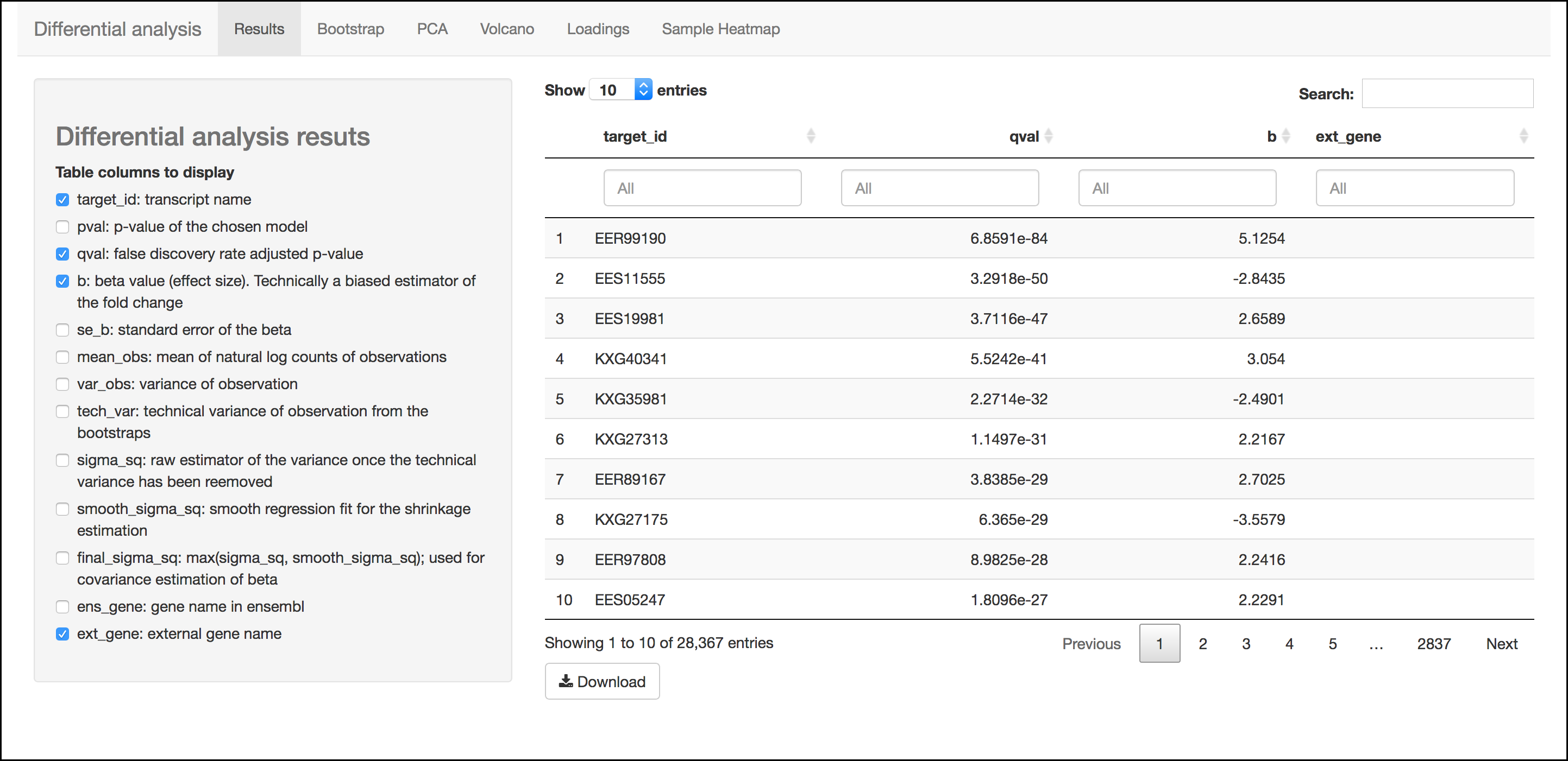
This menu is an interactive table of your results. You can choose which columns to display in the table using the checkboxes on the left of the screen. Several important values selected by default include:
- Target_id: This is the name of the transcript (gene) from the selected reference transcriptome.
- qval: This is a corrected (for multiple testing) p-value indicating the significance test of differential abundance. Lower numbers indicate greater significance.
- b: This is an estimate of the fold change between the conditions
- ext_gene: If available, these are gene names pulled from Ensemble
Tip
Click the `Download`{.interpreted-text role="guilabel"} button to download these results.
Bootstrap
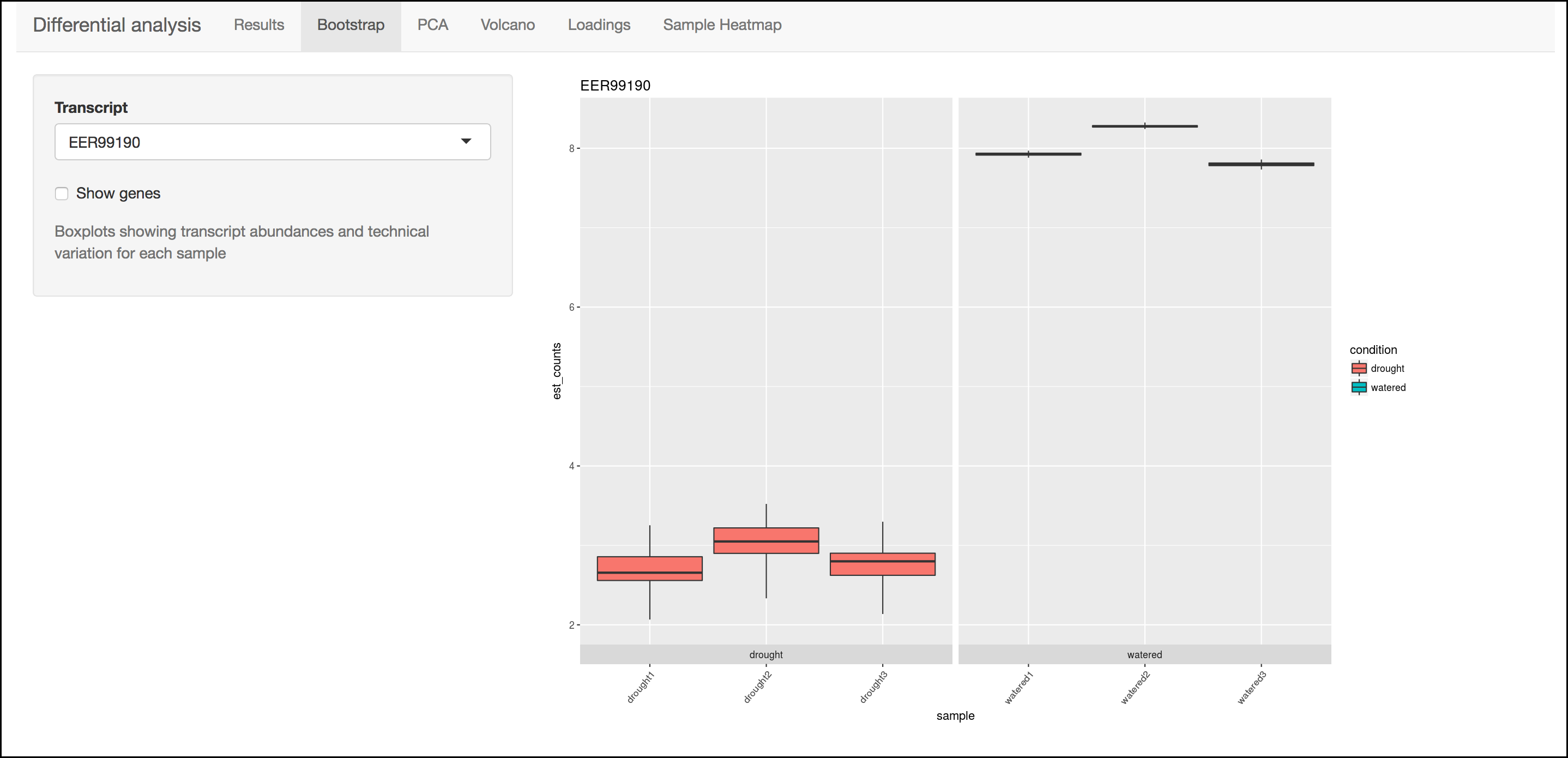
This menu will display a box plot that indicates the difference in expression between conditions. The box plots themselves indicate variation between replicates as estimated by bootstrap sampling of the reads. A dropbox enables you to select any transcript. Clicking the "Show genes" will load alternative gene names if available.
Tip
Right-click a graph to download this and other images.
PCA
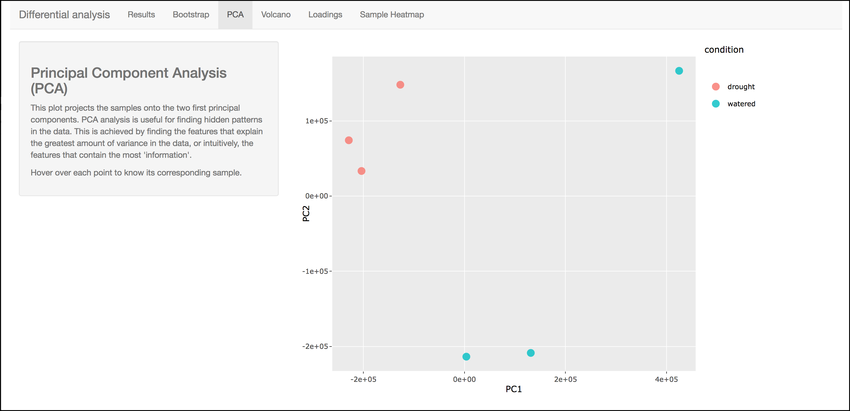
This graph displays principle components of each of the conditions/replicates. In general replicates of the same condition should cluster closely together.
Volcano Plot
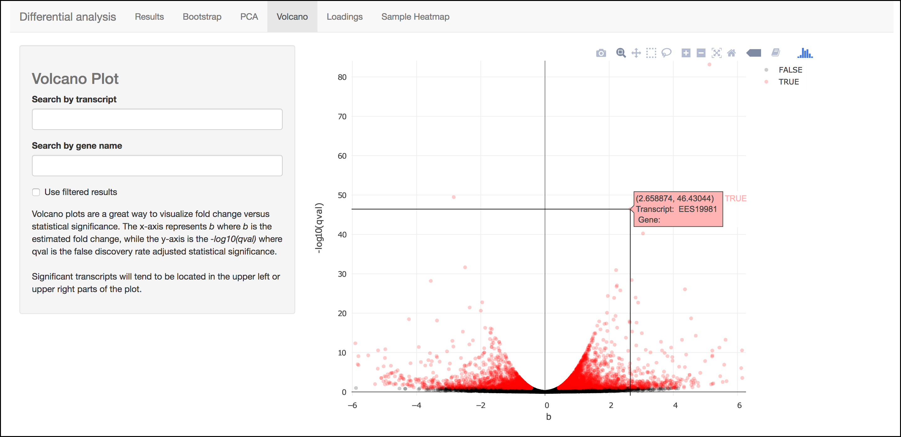
This scatter plot displays all transcripts colored by significance of differential abundance. You may also use menu on the left of the screen to highlight specific genes/transcripts or previously set filters from the results menu.
Loadings
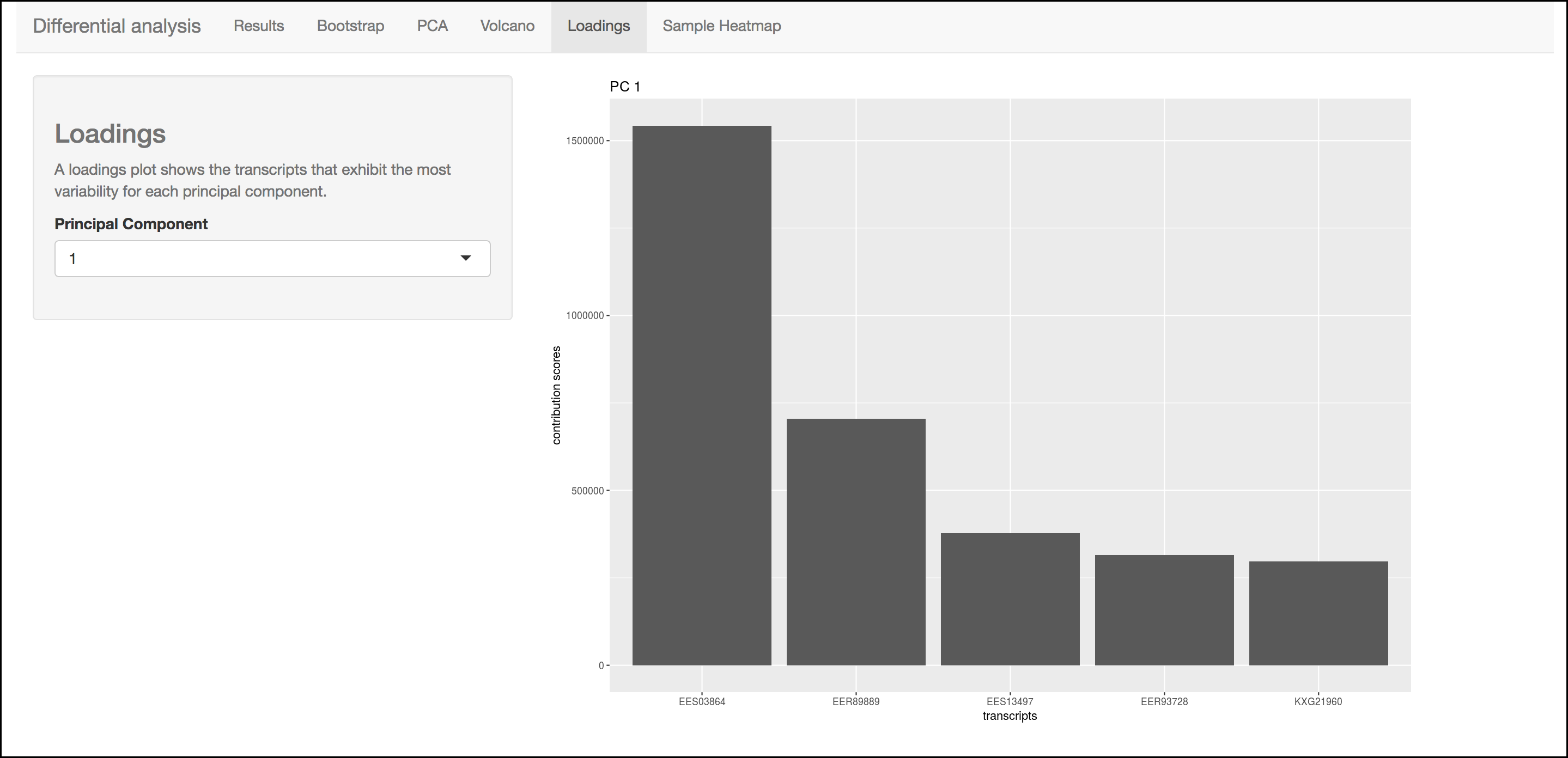
This barplot indicates which genes/transcripts explain most of the variance computed in the principle components analysis.
Heatmap
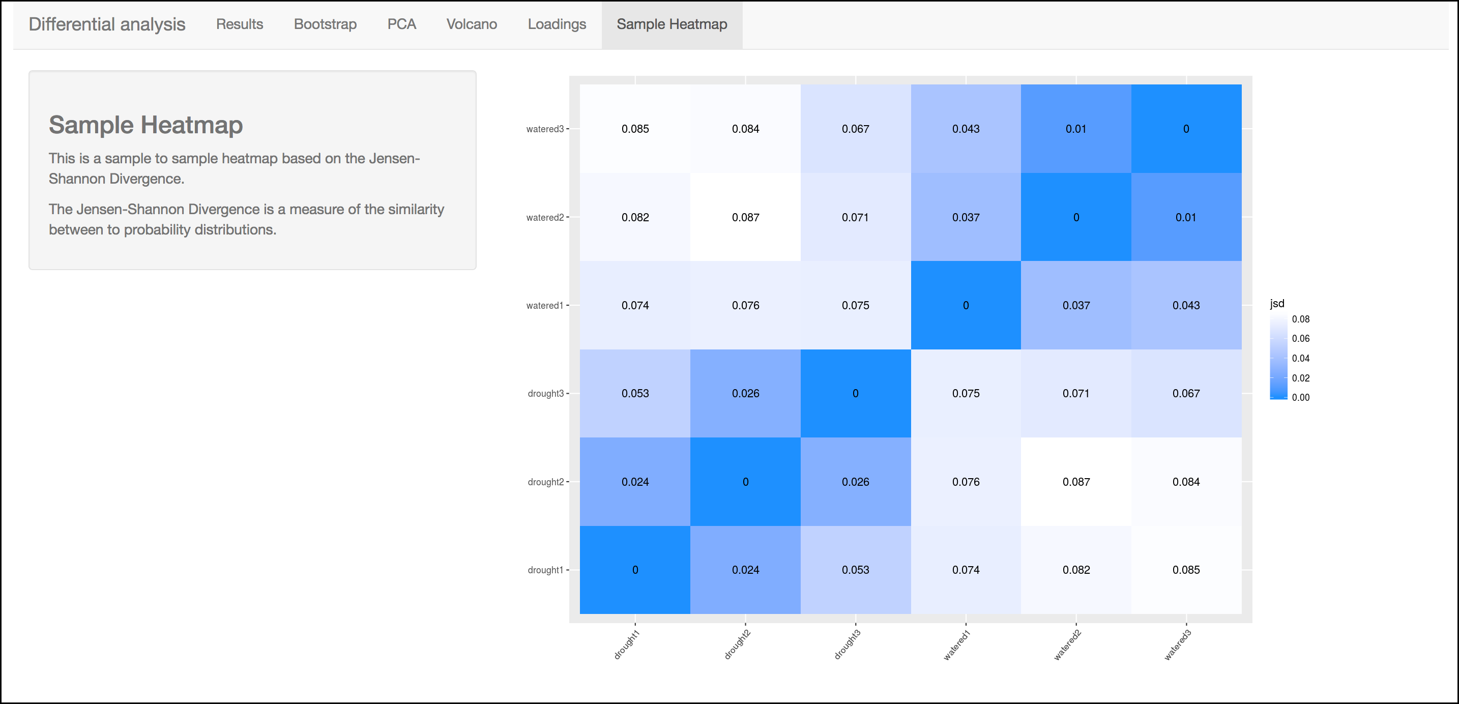
This heatmap gives a measure of the similarity between the possible comparison of the samples and their replicates.
Summary: Together, Kallisto and Sleuth are quick, powerful ways to analyze RNA-Seq data.
Walkthrough of DNA Subway Purple Line (beta testing documentation)
BETA RELEASE
The Purple line is in beta release. Please send feedback to [DNALC Admin](mailto:dnalcadmin@cshl.edu).
The Purple Line provides the capability for analysis of microbiome and eDNA (environmental DNA) by implementing a simplified version of the QIIME 2 (pronounced "chime two") workflow. Using the Purple Line, you can analyze uploaded high throughput sequencing reads to identify species in microbial or environmental DNA samples.
Metabarcoding uses high-throughput sequencing to analyze hundreds of thousands of DNA barcodes from complex mixtures of DNA. In a typical experiment, DNA is isolated from sterile swabs or material taken from different environmental locations or conditions. PCR is used to amplify a variable region, such as COI, or 12S or 16S ribosomal RNA genes, and sequence reads identify the variety and abundance of species from different samples. The analysis requires specialized software, such as QIIME 2.
The Purple Line integrates sequence data and metadata imported from CyVerse's Data Store, demultiplexing of samples, quality control, and taxonomic identification and quantitation. Once sequences are analyzed, the results can be visualized to allow comparisons between samples and different conditions summarized in the metadata.
Some things to remember about the platform
- You must be a registered CyVerse user to use Purple Line (register for a CyVerse account at user.cyverse.org).
- The Purple line was designed to make microbiome/eDNA data analysis "simple". However, we ask that users very carefully and thoughtfully decide what "jobs" they want to submit.
- A single Purple Line project may take hours to process since HPC computing is subject to queues which may support hundreds of other jobs. These systems also undergo regular maintenance and are subject to periodic disruption.
- DNA Subway implements the QIIME 2 software. This software is in continual development. Our version may not be the most current, and our documentation and explanation is not meant to replace the full QIIME 2 documentation.
- We have made design decisions to create a straightforward classroom-friendly workflow. While this Subway Line does not have all possible features of QIIME 2, we purpose to cover important concepts behind microbiome and eDNA analysis.
- You may work with up to 96 samples (e.g. 192 paired files or 96 single read files) in a Purple line project.
Sample Data: How to use provided sample data
In this guide, we will use a microbiome dataset (*"ubiome-test-data"*) collected from various
water sources in Montana (down-sampled and de-identified).Where
appropriate, a note (in this orange colored background) in the
instructions will indicate which options to select to make use of this
provided dataset.
DNA Subway Purple Line - Metadata file and Sequencing Prerequisites
If you are generating data for a project (i.e. sequencing samples), you will need to provide the sequencing data (fastq files) as well as a metadata file that describes the data contained in these sequencing files. This metadata must conform to strict guidelines, or analyses will fail. QIIME 2 metadata is stored in a TSV (tab-separated values) file. These files typically have a .tsv or .txt file extension, though it doesn't matter to QIIME 2 what file extension is used. TSV files are simple text files used to store tabular data, and the format is supported by many types of software, such as editing, importing, and exporting from spreadsheet programs and databases. Thus, it's usually straightforward to manipulate QIIME 2 metadata using the software of your choosing. If in doubt, we recommend using a spreadsheet program such as Microsoft Excel or Google Sheets to edit and export your metadata files.
Handling Project Metadata
Before you create your project, you will have generated metadata (as described above) for your project. You have two options for preparing this metadata to ensure that it conforms to the required QIIME2 parameters. The file must be validated (which you can do on your own or using Subway). If there are errors in your file (this is common), they must be fixed.
Formatting Your Metadata
**Leading and trailing whitespace characters**

If any cell in the metadata contains leading or trailing whitespace
characters (e.g. spaces, tabs), those characters will be ignored when
the file is loaded. Thus, leading and trailing whitespace characters
are not significant, so cells containing the values 'gut' and ' gut' are equivalent. This rule is applied before any other rules
described below

**ID column**

The first column MUST be the ID column name (i.e. ID header) and the
first line of this column should be #SampleID or one of a few
alternative.
-   Case-insensitive: id; sampleid; sample id; sample-id; featureid;
    feature id; feature-id.
-   Case-sensitive: #SampleID; #Sample ID; #OTUID; #OTU ID;
    sample_name

**Sample IDs**

For the sample IDs, there are some simple rules to comply with QIIME 2
requirements:

-   IDs may consist of any Unicode characters, with the exception
    that IDs must not start with the pound sign (#), as those rows
    would be interpreted as comments and ignored. IDs cannot be
    empty (i.e. they must consist of at least one character).
-   IDs must be unique (exact string matching is performed to detect
    duplicates).
-   At least one ID must be present in the file.
-   IDs cannot use any of the reserved ID column names (the sample
    ID names, above).
-   The ID column can optionally be followed by additional columns
    defining metadata associated with each sample or feature ID.
    Metadata files are not required to have additional metadata
    columns, so a file containing only an ID column is a valid QIIME
    2 metadata file.

**Column names**

-   May consist of any Unicode characters.
-   Cannot be empty (i.e. column names must consist of at least one
    character).
-   Must be unique (exact string matching is performed to detect
    duplicates).
-   Column names cannot use any of the reserved ID column names.

**Column values**

-   May consist of any Unicode characters.
-   Empty cells represent missing data. Note that cells consisting
    solely of whitespace characters are also interpreted as missing
    data.

QIIME 2 currently supports categorical and numeric metadata columns.
By default, QIIME 2 will attempt to infer the type of each metadata
column: if the column consists only of numbers or missing data, the
column is inferred to be numeric. Otherwise, if the column contains
any non-numeric values, the column is inferred to be categorical.
Missing data (i.e. empty cells) are supported in categorical columns
as well as numeric columns. For more details, and for how to define
the nature of the data when needed, see the [QIIME 2 metadata documentation](https://docs.qiime2.org/2019.10/tutorials/metadata/).
Working with an existing metadata file
Tip
If you have your own metadata file, it will still need to be validated once uploaded to DNA Subway.
Using a spreadsheet editor, create a metadata sheet that provides descriptions of the sequencing files used in your experiment. Export this file as a tab-delimited .txt or .tsv file. following the QIIME 2 metadata documentation](https://docs.qiime2.org/2019.10/tutorials/metadata/) recommendations. (Optional: if you using your own metadata file you can validate it using DNA Subway and or online QIIME2 validator Keemei).
Tip
See an example metadata file used for our sample data here: metadata file. Click the Download button on the
linked page to download and examine the file. (Note: This is an
Excel version of the metadata file, you must save Excel files as .TSV
(tab-separated) to be compatible with the QIIME 2 workflow.)
Creating a metadata file using DNA Subway
See DNA Subway Purple Line - Metadata and QC section C.
DNA Subway Purple Line - Create a Microbiome Analysis Project
A. Create a project in Subway
- Log-in to DNA Subway (unregistered users may NOT use Purple Line, register for a CyVerse account at user.cyverse.org.
- Click the purple square ("Microbiome Analysis") to begin a project.
-
For 'Select Project Type' select either Single End Reads or Paired End Reads
Sample Data
*"ubiome-test-data"* dataset: Select **Single End Reads**- For 'Select File Format' select the format the corresponds to your sequence metadata.
Sample Data
*"ubiome-test-data"* dataset: Select **Illumina Casava 1.8**Tip
Typically, microbiome/eDNA will be in the form of multiplexed FastQ sequences. We support the following formats: - [Illumina Casava 1.8](http://illumina.bioinfo.ucr.edu/ht/documentation/data-analysis-docs/CASAVA-FASTQ.pdf/at_download/file)- Enter a project title, and description; click
Continue.
B. Upload read data to CyVerse Data Store
The sequence read files used in these experiments are too large to
upload using the Subway interface. You must upload your files (Note: Only .fastq.gz files are accepted) directly to the CyVerse Data Store:
- Upload your
- FASTQ sequence reads; Note: Only
.fastq.gzfiles are accepted. - Sample metadata file (.tsv or .txt formatted according to QIIME 2 Metadata documentation) to the CyVerse Data Store using Cyberduck. See instructions: CyVerse Data Store Guide.
- FASTQ sequence reads; Note: Only
(Optional: You can edit and change metadata using the Subway interface in the [Manage data]step once the project is created.)
DNA Subway Purple Line - Metadata and QC
A. Select files using Manage Data
-
Click on the 'Manage data stop: this opens a window where you can add your FASTQ (up to 192 paired files or 96 single read files) and metadata files. Click
+Add from CyVerseto add the FASTQ files uploaded to the CyVerse Data Store. Select your files and then clickAdd selected files{.interpreted-text role="guilabel"} orAdd all FASTQ files in this directory{.interpreted-text role="guilabel"} as appropriate. Note: Only.fastq.gzfiles are accepted.Sample Data
*"ubiome-test-data"* dataset: Navigate to: Shared Data > SEPA_microbiome_2016 > **ubiome-test-data** and click `Add all FASTQ files in this directory`{.interpreted-text role="guilabel"}
2. To add your metadata file you may use one of three options: - Add from CyVerse: Add a metadata file you have uploaded to CyVerse Data store - Upload locally: Directly upload a metadata file from your local computer - Create New: Create a new metadata file using DNA Subway
Creating a metadata file using DNA Subway
You can create a metadata file using DNA Subway. Creating the file
step-by-step will help you to avoid metadata errors. Be sure you
have consulted the [QIIME 2 documentation](https://docs.qiime2.org/2019.10/tutorials/metadata/) so you can anticipate what the required fields
are. To use this feature under in the 'Manage data' step under
'Metadata Files' click `Create new`{.interpreted-text role="guilabel"}
**Sample IDs and adding/removing samples**
These are unique IDs for each of your samples.
All metadata files must have a column called **#SampleID**. Click
`+Add samples`{.interpreted-text role="guilabel"} to add additional
rows. In the Subway form, these will be unique, arbitrary names
(roughly corresponding to well-positions on a 96-well microplate).
You can change these (including pasting in sample names from an
existing spreadsheet).
{width="450px" height="250px"}
Right-clicking on a row number allows you to remove or insert rows.
{width="450px" height="250px"}
**Adding columns, managing sample descriptions and data types**
The very **last** column must be a sample description. You can click
the arrow on the right of this column to add a new column (which
will be added to the left). Column names must be unique, must not be
empty, cannot contain whitespace, can contain a maximum of 32
characters, cannot match a reserved column name. Notice that when
you click on a column name it is colored -pink for columns that have
numeric data (e.g. measurements) and cyan for everything else (e.g.
categorical descriptions in the form of words (i.e. strings)).
Clicking a column name will allow you to change its type.
{width="450px" height="250px"}
**Handling errors**
If you violate one of the rules for metadata formatting, the entry
will turn red. Consult the help and or the [QIIME 2 documentation](https://docs.qiime2.org/2019.10/tutorials/metadata/) to correct the error.
{width="450px" height="250px"}
Click `Save`{.interpreted-text role="guilabel"} to save your
metadata file, and close the window.
Sample Data
*"ubiome-test-data"* dataset: <br>
Click `Add from CyVerse`{.interpreted-text role="guilabel"}Navigate to: Shared Data > SEPA_microbiome_2016 > **ubiome-test-data**
Select the **mappingfile_MT_corrected.tsv** and then click `Add selected files`{.interpreted-text role="guilabel"}.
3. As needed, you can edit or rename your metadata file. Before
proceeding, you must validate your metadata file. To validate,
click the "validate" link to the right of the metadata file you
wish to check. Once the validation completed, click Run to proceed. If you have
errors, you will be presented with an Edit button so that you can return to the file and
edit.
B. Demultiplex reads
At this step, reads will be grouped according to the sample metadata. This includes separating reads according to their index sequences if this was not done prior to running the Purple Line. For demultiplexing based on index sequences, the index sequences must be defined in the metadata file.
Note
Even if your files were previously demultimplexed (as will generally
be the case with Illumina data) you must still complete this step to
have your sequence read files appropriately associated with metadata.
1. Click the 'Demultiplex reads' and choose a number of reads to sample. When the job has completed click Demultiplexing Summary to view your results. In 'Random sequences to sample for QC', enter a value (1000 is recommended),
Sample Data
*"ubiome-test-data"* dataset: Use the default of 1000 sequences
2. When demultiplexing is complete, you will generate a file (.qzv) click this link to view a visualization and statistics on the sequence and metadata for this project.
Tip
Several jobs on Purple Line will take several minutes to an hour
to complete. Each time you launch one of these steps you will get
a Job ID. You can click the `View job info`{.interpreted-text
role="guilabel"} button to see a detailed status and
diagnostic/error messages. If needed There is a [stop this job]{.title-ref} link at the bottom of the info page to cancel a
job.

!!! Note

        **QIIME2 Visualizations**

        One of the features of QIIME 2 are the variety of visualizations
        provided at several analysis steps. Although this guide will not
        cover every feature of every visualization, here are some
        important points to note.

        **QIIME2 View**: DNA Subway uses the QIIME 2 View plugin to
        display visualizations. Like the standalone QIIME 2
        software, you can navigate menus, and interact with several
        visualizations. Importantly, many files and visualizations
        can be directly download for your use outside of DNA Subway,
        including in report generation, or in your custom QIIME 2
        analyses. You can view downloaded .qza or .qzv files at [view.qiime2.org](https://view.qiime2.org/).
Quality Graphs Explained
After demultiplexing, you will be presented with a visualization
that displays the following tables and graphs:
**Overview Tab**
- *Demultiplexed sequence counts summary*: For each of the
fastq files (each of which may generally correspond to a
single sample), you are presented with comparative
statistics on the number of sequences present. This is
followed by a histogram that plots number of sequences by
the number of samples. <br>
- *Per-sample sequence counts*: These are the actual counts
of sequences per sample as indicated by the sample names
you provided in your metadata sheet.
{width="450px" height="250px"}
**Interactive Quality Plot**
This is an interactive plot that gives you an average quality
(y-axis) by the position along the read (x-axis). This box plot
is derived from a random sampling of a subset of sequences. The
number of sequences sampled will be indicated in the plot
caption. You can use your mouse drag and zoom in to regions on
the plot. Double-click your mouse to zoom out.
{width="450px" height="250px"}
3. Click the "Interactive Quality Plot" tab to view a histogram of sequence quality. Use this plot at the tip below to determine a location to trim.
Tips on trimming for sequence quality
On the Interactive Quality Plot you are shown an histogram, plotting
the average quality (x axis) [Phred score](https://en.wikipedia.org/wiki/Phred_quality_score) vs. the position on the read (y axis) in base pairs for a **subsample** of reads.
**Zooming to determine 3' trim location**
Click and drag your mouse around a collection of base pair positions
you wish to examine. Clicking on a given histogram bar will also
generate a text report and metrics in the table below the chart. Using
these metrics, you can choose a position to trim on the right side
(e.g. 3' end of the sequence read). The 5' (left trim) is specific
to your choice of primers and sequencing adaptors (e.g. the sum of the
adaptor sequence you expect to be attached to the 5' end of the
read). Poor quality metrics will generate a table colored in red, and
those base positions will also be colored red in the histogram.
Double-clicking will return the histogram to its original level of
zoom.
**Example plots**
It is important to maximize the length of the reads while minimizing
the use of low quality base calls. To this end, a good guideline is to
trim the right end of reads to a length where the 25th percentile is
at a quality score of 25 or more. However, the length of trimming will
depend on the quality of the sequence, so you may have to use a lower
quality threshold to retain enough sequence for informative sequence
searches and alignments. This may require multiple runs of the
analysis to find the optimal trim length for your data.
*Quality drops significantly at base 35*
{width="400px" height="250px"}
*Improved quality sequence*
{width="400px" height="250px"}
C. Use DADA2 for Trimming and Error-correction of Reads
It is important to only work with high quality data. This step will generate a sequence quality histogram which can be used to determine parameter for trimming.
-
Click 'DADA2' and choose the metadata file corresponding to the samples you wish to analyze. Then choose values for trimming of the reads. For "trimLeft" (the position starting from the left you wish to trim) and "TruncLen" (this is the position where reads should be trimmed, truncating the 3' end of the read. Reads shorter than this length will be discarded). Finally, click
Trim reads.Sample Data
*"ubiome-test-data"* dataset: Based on the histogram for our sample, we recommend the following parameters:

-   **trimLeft: 17** (this is specific to primers and adaptors in
    this experiment)
-   **TruncLen: 200** (this is where low quality sequence begins, in
    this case because our sequence length is lower than the expected
    read length)
D. Check Results of Trimming Once trimming is complete, the following outputs are expected:
-
Click on DADA2 and then click on the links in the Results table to examine results.
-
Trim Table (Metric summary, Frequency per sample, Frequency per feature): Summarizes the dataset post-trimming including the number of samples and the number of features per sample. The "Interactive Sample Detail" tab contains a sampling depth tool that will be used in computation of the core matrix.
Note
**You will use the maximum frequency value for the Alpha rarefaction step** So you may wish to record this value now for the DNA Subway 'Clustering sequences' step. -
Stats: Sequencing statistics for each of the sample IDs described in the original metadata file.
- Representative Sequences (Sequence Length Statistics, Seven-Number Summary of Sequence Lengths, Sequence Table): This table contains a listing of features observed in the sequence data, as well as the DNA sequence that defines a feature. Clicking on the DNA sequence will submit that sequence for BLAST at NCBI in a separate browser tab.
The feature table contains two columns output by DADA2. DADA2 (Divisive Amplicon Denoising Algorithm 2) determines what sequences are in the samples. DADA2 filters the sequences and identifies probable amplification or sequencing errors, filters out chimeric reads, and can pair forward and reverse reads to create the best representation of the sequences actually found in the samples and eliminating erroneous sequences.
- Feature ID: A unique identifier for sequences.
- Sequence: A DNA Sequence associated with each identifier.
Clicking on any given sequence will initiate at BLAST search on the NCBI website. Click "View report" on the BLAST search that opens in a new web browser tab to obtain your results. Keep in mind that if your sequences are short (due to read length or trimming) many BLAST searches may not return significant results.
Tip
Although the term "feature" can (unfortunately) [have many meanings](https://forum.qiime2.org/t/what-is-a-feature-exactly/2201) as used by the
QIIME2 documentation, unless otherwise noted in this documentation
it can be thought of as an OTU ([Operational Taxonomic Unit](https://en.wikipedia.org/wiki/Operational_taxonomic_unit)); another substitution for the word
species. OTU is a convenient and common terminology for referring to
an unclassified or undetermined species. Ultimately, we are
attempting to identify an organism from a sample of DNA which may
not be informative enough to reach a definitive conclusion.
Tip
If you want to redo the DADA2 step with different parameters, click
the "New Job" tab on the upper left of a DADA2 window to submit a
new job. New jobs appear as tabs on Subway steps that are typically
run several times. You can go back an see these jobs which are
labeled with a job number.
{width="450px" height="250px"}
DNA Subway Purple Line - Alpha Rarefaction/Clustering Sequences
A. Alpha rarefaction
At this step, you can visualize summaries of the data. A feature table will generate summary statistics, including how many sequences are associated with each sample. Note that sample depth is limited to 100,000.
- Click on 'Alpha rarefaction'. Select "run" and designate the
minimum and maximum rarefaction depth. A minimum value should be
set at 1. The maximum value is specific to your data set. The
maximum value is specific to your data set. To determine what the
maximum value should be set to, open the "Trim Table" from the
"DADA2" step. You may not choose a value that is greater than
the maximum frequency per sample. In general, choosing a value
that is somewhere around the median frequency seems to work well,
but you may want to increase that value if the lines in the
resulting rarefaction plot don't appear to be leveling out, or
decrease that value if you seem to be losing many of your samples
due to low total frequencies closer to the minimum sampling depth
than the maximum sampling depth. Identify the maximum Sequence
Count value and enter that number as the maximum value. Click
Submit Job.
Note
Since you may want to try Alpha rarefaction using different
combinations of results from DADA2 trimming and your choice of
rarefaction depths, your trim (DADA2) jobs are displayed on the
left, and each new Alpha rarefaction setting will appear as a tab on
the top.
{width="450px" height="250px"}
Sample Data
*"ubiome-test-data"* dataset:
We recommend the following parameters:

-   **Min. rarefaction depth**: 1

-   **Max. rarefaction depth**: 2938
- Under 'Results' click on Alpha Rarefaction Plot to view the results.
Navigating Alpha Rarefaction graphs
Alpha rarefaction generates an interactive plot of species diversity by sampling depth by the categorical samplings described in your sample metadata. You can use dropdown menus to change metrics/conditions displayed and also export data as a CSV file.
DNA Subway Purple Line - Calculate Core Metrics/Alpha and Beta Diversity
At this stop, you will examine Alpha Diversity (the diversity of species/taxa present within a single sample) and Beta Diversity (a comparison of species/taxa diversity between two or more samples).
- Alpha diversity answers the question - "How many species are in a sample?"
- Beta diversity answer the question - "What are the differences in species between samples?"
A. Calculate core metrics
- Click on 'Core metrics' and then click the "run" link. Choose
a sampling depth based upon the "Sampling depth" tool (described
in Section D Step 1, in the Trim Table output; Interactive
Sample Detail tab). Choose an appropriate classifier (see
comments in the tip below) and click
Submit job.
Choosing Core metrics parameters
*Sampling Depth*

In downstream steps, you will need to choose a sampling depth for
your sample comparisons. You can choose by examining the table
generated at the **Trim reads** step. In the *Trim Table* output,
*Interactive Sample Detail* tab, use the "Sampling depth" tool to
explore how many sequences can be sampled during the Core matrix
computation. As you slide the bar to the right, more sequences are
sampled, but samples that do not have this many sequences will be
removed during analysis. The sampling depth affects the number of
sequences that will be analyzed for taxonomy in later steps: as the
sampling depth increases, a greater representation of the sequences
will be analyzed. However, high sampling depth could exclude
important samples, so a balance between depth and retaining samples
in the analysis must be found.

*Classifier*

Choose a classifier pertaining to your experiment type.

-   **Microbiome** choose **Greengenes (515F/806R)** or **Greengenes
    (full sequences)** or **Sliva (16S rRNA)** classifier
-   **eDNA** experiment with marine fishes you may elect to choose
    the **Fish 12S/ecoPrimer** classifier
Sample Data
*"ubiome-test-data"* dataset:
We recommend the following parameters:

-   **Sampling Depth**: 3000

-   **Classifier**: Grenegenes (full sequences)
B. Examine alpha and beta diversity
-
When core metrics is complete, you should generate several visualization results. Click each of the following to get access:
-
Alpha Diversity:
-
Pielou's Evenness
-
Alpha Correlation: Measure of community evenness using correlation tests
-
Group Significance: Analysis of differences between features across group
-
-
Faith's Phylogenetic Diversity
-
Alpha Correlation: Faith Phylogenetic Diversity (a measure of community richness) with correlation tests
-
Group Significance: Faith Phylogenetic Diversity ( a measure of community richness)
-
-
-
Beta Diversity:
-
Bray-Curtis Distance
Bray-Curtis is a metric for describing the dissimilarity of species in an ecological sampling. - Bioenv: Bray-Curtis test metrics
- Emperor: Interactive PCoA plot of Bray-Curtis metrics
-
Jaccard Distance
- Emperor: Interactive PCoA plot calculated by Jaccard similarity index.
-
Unweighted UniFrac Distance
UniFrac is a metric for describing the similarity of a biological community, taking into account the relatedness of community members.
-
Bioenv: UniFrac test metrics
-
Emperor: Unweighted interactive PCoA plot
-
-
Weighted UniFrac Distance
Unweighted UniFrac removes the effect of low-abundance features in the calculation of principal components.
- Emperor: Weighted interactive PCoA plot of UniFrac.
-
-
Tip
**Emperor Plots**
These plots are all interactive three-dimensional plots of an
analysis using [principal components](https://en.wikipedia.org/wiki/Principal_component_analysis).
**Customization**
You can customize Emperor plots, including altering the color of
and shape points, axes, and other parameters. You can also export
images from this visualization.
{width="550px" height="300px"}
**Bioenv**
These plots are tables of tests and descriptive metrics.
C. Taxonomic Diversity:
Taxonomic diversity is at the heart of many analyses. We suggest consulting the QIIME taxonomy overview for a detailed explanation of how QIIME2 calculates taxonomy and additional features of QIIME2 you may wish to explore beyond the functionalities DNA Subway has included.
-
Bar Plots
-
An interactive stacked bar plot of species diversity. Dropdown menus allow you to color by seven taxonomic levels 1) kingdom, 2) phylum, 3) class, 4) order, 5), family, 6) genus, 7) species. Plots can be further arranged/filtered/sorted accoridng to characteristics in the sample metadata. You may also download images and data used to create the barpot visualization.
-
-
Taxonomy
- A table indicating the identified "features", their taxa, and an indication of confidence.
You can download and interact with any of the available plots.
D. Calculate differential abundance
- Click on the 'Differential abundance' stop. Then click on the
"Submit new "Differential abundance" job" link. Choose a
metadata category to group by, and a level of taxonomy to
summarize by. Then click
&submit job{.interpreted-text role="guilabel"}.
Sample Data
*"ubiome-test-data"* dataset:

We recommend the following parameters:

-   **Group data by**: CollectionMethod

-   **Level of taxonomy to summarize**: 5
Tip
Download the provided CSV files so that you can generate customized plots.
DNA Subway Purple Line - Visualize data with PiCrust and PhyloSeq
Under Development